18  Agricultural Production: Positive vs. Negative Surprise Shocks (LP)

Objectives

Estimate response functions of agricultural production following a positive or negative surprise weather shock, using Local Projections. The surprise weather shocks are defined following Natoli (2024).

\[ \definecolor{bayesred}{RGB}{147, 30, 24} \definecolor{bayesblue}{RGB}{32, 35, 91} \definecolor{bayesorange}{RGB}{218, 120, 1} \definecolor{grey}{RGB}{128, 128, 128} \definecolor{couleur1}{RGB}{0,163,137} \definecolor{couleur2}{RGB}{255,124,0} \definecolor{couleur3}{RGB}{0, 110, 158} \definecolor{coul1}{RGB}{255,37,0} \definecolor{coul2}{RGB}{242,173,0} \definecolor{col_neg}{RGB}{155, 191, 221} \definecolor{col_pos}{RGB}{255, 128, 106} \definecolor{wongBlack}{RGB}{0,0,0} \definecolor{wongLightBlue}{RGB}{86, 180, 233} \definecolor{wongGold}{RGB}{230, 159, 0} \definecolor{wongGreen}{RGB}{0, 158, 115} \definecolor{wongYellow}{RGB}{240, 228, 66} \definecolor{wongBlue}{RGB}{0, 114, 178} \definecolor{wongOrange}{RGB}{213, 94, 0} \definecolor{wongPurple}{RGB}{204, 121, 167} \definecolor{IBMPurple}{RGB}{120, 94, 240} \definecolor{IBMMagenta}{RGB}{220, 38, 127} \]

This chapter uses Jordà (2005) Local Projection framework to measure how sensitive agricultural output is to exogenous changes in the weather. It complements Chapter 7 by testing alternative weather shock definitions.

Reminder

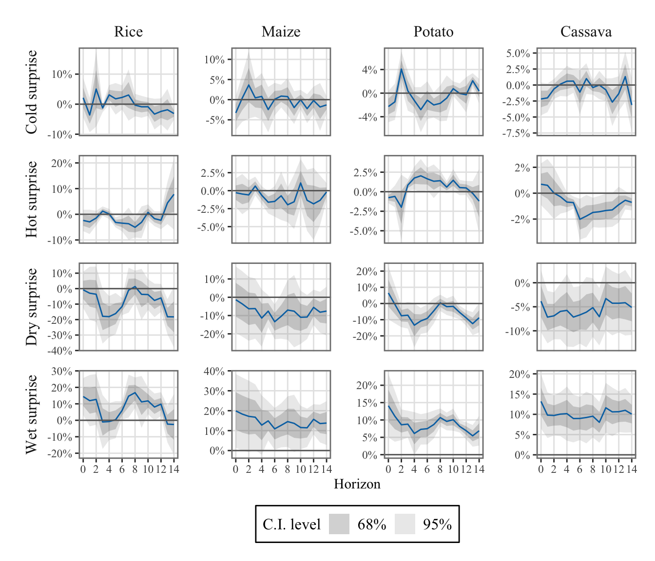
To differentiate the effects of positive and negative shocks, we defined two indicators for both temperature and precipitation: one for positive shocks and another for negative shocks (see Section 1.4.3).

The idea is to compare the realized temperatures (or precipitation) in a given month \(m\) of year \(y\) at location \(\ell\) with expected temperatures (precipitation) based on observations from the same month in previous years at the same location. The difference is defined as a surprise shock.

For days hotter (wetter) than expected, the shock in cell \(\ell\) is defined as: \[ \begin{align} W^{(+)}_{\ell,y,m, c} = \underbrace{\sum_{d=1}^{n_m} \mathrm{1}(\mathcal{W}_{\ell,y,m,d} > \text{ut}_{\ell,y,m, c})}_{\text{Climate realization}} - \underbrace{\frac{1}{5}\sum_{k=1}^{5}\sum_{d=1}^{n_m} \mathrm{1}(\mathcal{W}_{\ell,y-k,m,d} > \text{ut}_{\ell,y,m, c})}_{\text{Expected realization}}, \end{align} \] where \(\mathcal{W}_{\ell,y,m,d}\) is the daily average temperature (or total rainfall), \(n_m\) is the number of days in month \(m\), and \(\text{ut}^{\mathcal{w}}_{\ell,y,m, c}\) is the threshold for hot days for crop \(c\).

Similarly, cold (dry) shocks are defined as: \[ \begin{align} W^{(-)}_{\ell,y,m,c} = \sum_{d=1}^{n_m} \mathrm{1}(\mathcal{W}_{\ell,y,m,d} < \text{lt}_{\ell,y,m, c}) - \frac{1}{5}\sum_{k=1}^{5}\sum_{d=1}^{n_m} \mathrm{1}(\mathcal{W}_{\ell,y-k,m,d} < \text{lt}_{\ell,y,m,c}), \end{align} \] where \(\text{lt}_{\ell,y,m,c}\) is the crop-specific threshold for cold days.

Thresholds \(\text{ut}_{\ell,y,m,c}\) and \(\text{lt}_{\ell,y,m,c}\) are based on the 90th and 10th percentiles of temperatures (precipitation) observed during month \(m\) over the past five years. The sample of past observation is denoted as \(\boldsymbol{W}_{\ell,y,d} = \left\{\{\mathcal{W}_{\ell,y-1,m,d}\}_{d=1}^{n_m}, \{\mathcal{W}_{c,y-2,m,d}\}_{d=1}^{n_m}, \ldots, \{\mathcal{W}_{c,y-5,m,d}\}_{d=1}^{n_m}\}\right\}\).

For temperature shocks, the thresholds are defined as follows: \[ \begin{align} \text{ut}_{\ell,y,m,c} &= \max\{P_{90}(\boldsymbol{T}_{\ell,y,d}), \tau_{\text{upper},c}\}\\ \text{lt}_{\ell,y,m,c} &= \min\{P_{10}(\boldsymbol{T}_{\ell,y,d}), \tau_{\text{lower}},c\} \end{align} \] with \(\tau_{\text{upper},c} = 29^\circ\text{C}\) for rice and maize, \(30^\circ\text{C}\) for potatoes and cassava, and \(\tau_{\text{lower},c} = 8^\circ\text{C}\) for rice and maize, \(10^\circ\text{C}\) for potatoes and cassava.

For precipitation shocks, the thresholds are defined using the percentiles of past values only:% \[ \begin{align} \text{ut}_{\ell,y,m,c} &= P_{90}(\boldsymbol{P}_{\ell,y,d})\\ \text{lt}_{\ell,y,m,c} &= P_{10}(\boldsymbol{P}_{\ell,y,d}) \end{align} \]

Positive values of \(\mathcal{W}^{(+)}_{\ell,y,m,c}\) represent days that are hotter (or wetter) than expected, while positive values of \(\mathcal{W}^{(-)}_{\ell,y,m,c}\) represent days that are colder (or drier) than expected.

The values were aggregated at the monthly regional level (see Chapter 1).

library(tidyverse)
── Attaching core tidyverse packages ──────────────────────── tidyverse 2.0.0 ──
✔ dplyr     1.1.4     ✔ readr     2.1.5
✔ forcats   1.0.0     ✔ stringr   1.5.1
✔ ggplot2   3.5.1     ✔ tibble    3.2.1
✔ lubridate 1.9.3     ✔ tidyr     1.3.1
✔ purrr     1.0.2     
── Conflicts ────────────────────────────────────────── tidyverse_conflicts() ──
✖ dplyr::filter() masks stats::filter()
✖ dplyr::lag()    masks stats::lag()
ℹ Use the conflicted package (<http://conflicted.r-lib.org/>) to force all conflicts to become errors
library(fastDummies)
Thank you for using fastDummies!
To acknowledge our work, please cite the package:
Kaplan, J. & Schlegel, B. (2023). fastDummies: Fast Creation of Dummy (Binary) Columns and Rows from Categorical Variables. Version 1.7.1. URL: https://github.com/jacobkap/fastDummies, https://jacobkap.github.io/fastDummies/.

The data can be loaded (see Chapter 5)

load("../data/output/df_lp.rda")
df
# A tibble: 14,040 × 116
   product_eng region_id month date       y_new y_dev_pct y_new_normalized     y
   <chr>       <fct>     <dbl> <date>     <dbl>     <dbl>            <dbl> <dbl>
 1 Cassava     1             1 2001-01-01 5322     -0.452            0.548 0.527
 2 Cassava     1             2 2001-02-01 4388     -0.555            0.445 0.402
 3 Cassava     1             3 2001-03-01 5664.    -0.455            0.545 0.480
 4 Cassava     1             4 2001-04-01 5664.    -0.434            0.566 0.486
 5 Cassava     1             5 2001-05-01 5099     -0.534            0.466 0.370
 6 Cassava     1             6 2001-06-01 5537     -0.544            0.456 0.308
 7 Cassava     1             7 2001-07-01 5537     -0.523            0.477 0.335
 8 Cassava     1             8 2001-08-01 5993     -0.481            0.519 0.346
 9 Cassava     1             9 2001-09-01 5622.    -0.519            0.481 0.273
10 Cassava     1            10 2001-10-01 5622.    -0.464            0.536 0.315
# ℹ 14,030 more rows
# ℹ 108 more variables: t <int>, region <chr>, product <chr>, ln_prices <dbl>,
#   ln_produc <dbl>, year <dbl>, Value_prod <dbl>, surf_m <dbl>,
#   Value_surfR <dbl>, Value_prices <dbl>, campaign <dbl>,
#   campaign_plain <chr>, month_campaign <dbl>, surf_lag_calend <dbl>,
#   perc_product <dbl>, perc_product_mean <dbl>, diff_plant_harv <dbl>,
#   exposition <dbl>, exposition_trend <dbl>, exposition_detrended <dbl>, …

Some packages are needed, make sure that they are installed.

# install.packages("fastDummies")
# install.packages("imputeTS")
# install.packages("ggh4x")
# install.packages("mFilter")
# install.packages("pbapply")
# install.packages("latex2exp")
# install.packages("sandwich")

We load some useful functions:

# Functions useful to shape the data for local projections
source("../weatherperu/R/format_data.R")

# Load function in utils
source("../weatherperu/R/utils.R")

# Load detrending functions
source("../weatherperu/R/detrending.R")

Each row of df gives production data for a crop \(c\) in region \(i\) at time \(t\). The surprise weather shocks were computed using crop-specific thresholds. We need to create four variables for the surprise shocks: cold_surprise, hot_surprise, dry_surprise, wet_surprise. The values in these four columns must correspond to the shock defined using the crop-specific threshold.

df <- 
  df |> 
  mutate(
   cold_surprise = case_when(
     product_eng == "Rice" ~ cold_surprise_rice,
     product_eng == "Dent corn" ~ cold_surprise_maize,
     product_eng == "Potato" ~ cold_surprise_potato,
     product_eng == "Cassava" ~ cold_surprise_cassava,
     TRUE ~ NA_real_
   ),
   hot_surprise = case_when(
     product_eng == "Rice" ~ hot_surprise_rice,
     product_eng == "Dent corn" ~ hot_surprise_maize,
     product_eng == "Potato" ~ hot_surprise_potato,
     product_eng == "Cassava" ~ hot_surprise_cassava,
     TRUE ~ NA_real_
   ),
   dry_surprise = case_when(
     product_eng == "Rice" ~ dry_surprise_rice,
     product_eng == "Dent corn" ~ dry_surprise_maize,
     product_eng == "Potato" ~ dry_surprise_potato,
     product_eng == "Cassava" ~ dry_surprise_cassava,
     TRUE ~ NA_real_
   ),
   wet_surprise = case_when(
     product_eng == "Rice" ~ wet_surprise_rice,
     product_eng == "Dent corn" ~ wet_surprise_maize,
     product_eng == "Potato" ~ wet_surprise_potato,
     product_eng == "Cassava" ~ wet_surprise_cassava,
     TRUE ~ NA_real_
   )
  )

18.1 Linear Local Projections

In this section, we focus on estimating the Local Projections (Jordà 2005) to quantify the impact of weather on agricultural production. We use panel data, similar to the approach used in the study by Acevedo et al. (2020), and independently estimate models for each specific crop.

For a particular crop denoted as \(c\), the model can be expressed as follows: \[ \begin{aligned} \underbrace{y_{c,i,{\color{wongGold}t+h}}}_{\text{Production}} = & {\color{wongOrange}\beta_{c,{\color{wongGold}h}}^{{\color{wongPurple}HotSurprise}}} {\color{wongPurple}{\text{HotSurprise}^{+}_{i,{\color{wongGold}t}}}} + {\color{wongOrange}\beta_{c,{\color{wongGold}h}}^{{\color{wongPurple}ColdSurprise}}} {\color{wongPurple}{\text{ColdSurprise}^{+}_{i,{\color{wongGold}t}}}}\\ & + {\color{wongOrange}\beta_{c,{\color{wongGold}h}}^{{\color{wongPurple}DrySurprise}}} {\color{wongPurple}{\text{DrySurprise}^{+}_{i,{\color{wongGold}t}}}} + + {\color{wongOrange}\beta_{c,{\color{wongGold}h}}^{{\color{wongPurple}WetSurprise}}} {\color{wongPurple}{\text{WetSurprise}^{+}_{i,{\color{wongGold}t}}}}\\ &+\gamma_{c,i,h}\underbrace{X_{t}}_{\text{controls}} + \underbrace{\zeta_{c,i,h} \text{Trend}_{t} + \eta_{c,i,h} \text{Trend}^2_{t}}_{\text{regional monthly trend}} + \varepsilon_{c,i,t+h} \end{aligned} \tag{18.1}\]

Here, \(i\) represents the region, \(t\) represents the time, and \(h\) represents the horizon. The primary focus lies on estimating the coefficients associated with temperature surprise shocks and precipitation surprise shocks for different time horizons \(\color{wongGold}h=\{0,1,...,T_{c}\}\)

Note that we allow a crop regional monthly specific quadratic trend to be estimated.

18.1.1 Functions

The estimation functions presented in Chapter 7.1.1 can be sourced.

source("../weatherperu/R/estimations.R")

18.1.2 Estimation

To loop over the different crops, we can use the map() function. This function enables us to apply the estimate_linear_lp() function to each crop iteratively, facilitating the estimation process.

crops <- df$product_eng |> unique()
weather_variables <- c("cold_surprise", "hot_surprise", "dry_surprise", "wet_surprise")
control_variables <- c("rer_hp", "r_hp", "pi", "ind_prod", "ONI", "price_int_inf")
nb_h <- 14

The estimation (this code takes about a minute to run, we load results in this notebook):

resul_lp <- vector(mode = "list", length = length(crops))
for (i_crop in 1:length(crops)) {
  print(crops[i_crop])
  resul_lp[[i_crop]] <- estimate_linear_lp(
    df,
    horizons = nb_h,
    y_name = "y_new_normalized",
    group_name = "region_id",
    detrend = TRUE,
    add_month_fe = FALSE,
    add_intercept = FALSE,
    crop_name = crops[i_crop],
    control_names = control_variables,
    weather_names = weather_variables,
    std = "Cluster",
    # std = "nw",
    other_var_to_keep = "y_new"
  )
}
save(resul_lp, file = "output/resul_lp_surprise.rda")
load("../R/output/resul_lp_surprise.rda")

18.1.3 Results

We can visualize the Impulse Response Functions (IRFs) by plotting the estimated coefficients associated with the weather variables. These coefficients represent the impact of weather on agricultural production and can provide valuable insights into the dynamics of the system. By plotting the IRFs, we can gain a better understanding of the relationship between weather variables and the response of agricultural production over time.

The data for the graphs:

df_irfs_lp <- map(resul_lp, "coefs") |> 
  list_rbind() |> 
  filter(name %in% weather_variables) |> 
  mutate(
    shock_1_sd = value * std_shock,
    lower_95 = (value - qnorm(0.975) * std) * std_shock,
    upper_95 = (value + qnorm(0.975) * std) * std_shock,
    lower_68 = (value - qnorm(0.84)  * std) * std_shock,
    upper_68 = (value + qnorm(0.84)  * std) * std_shock
  ) |> 
  mutate(
    crop = factor(
      crop, 
      levels = c("Rice", "Dent corn", "Potato", "Cassava"),
      labels = c("Rice", "Maize", "Potato", "Cassava"))
  ) |> 
  mutate(
    name = factor(
      name,
      levels = c(
        "cold_surprise",
        "hot_surprise",
        "dry_surprise",
        "wet_surprise"
      ),
      labels = c(
        "Cold surprise", 
        "Hot surprise",
        "Dry surprise", 
        "Wet surprise"
      )
    )
  )

For the confidence intervals:

df_irfs_lp_ci <- 
  df_irfs_lp |> 
  select(horizon, crop, name, matches("^(lower)|^(upper)", perl = TRUE)) |> 
  pivot_longer(
    cols = matches("^(lower)|^(upper)", perl = TRUE),
    names_pattern = "(.*)_(95|68)$",
    names_to = c(".value", "level")
  ) |> 
  mutate(level = str_c(level, "%"))
ggplot() +
  geom_ribbon(
    data = df_irfs_lp_ci |> filter(horizon <= !!nb_h),
    mapping = aes(
      x = horizon,
      ymin = lower, ymax = upper, fill = level),
    alpha = .2
  ) +
  geom_line(
    data = df_irfs_lp |> filter(horizon <= !!nb_h),
    mapping = aes(x = horizon, y = shock_1_sd),
    colour = "#0072B2") +
  geom_hline(yintercept = 0, colour = "gray40") +
  ggh4x::facet_grid2(
    name~crop, scales = "free_y", 
    independent = "y", switch = "y") +
  scale_x_continuous(breaks = seq(0, nb_h, by = 2)) +
  scale_y_continuous(labels = scales::percent) +
  labs(x = "Horizon", y = NULL) +
  scale_fill_manual(
    "C.I. level", 
    values = c("68%" = "gray10", "95%" = "gray60")
  ) +
  theme_paper() +
  theme(strip.placement = "outside")
Figure 18.1: Agricultural production response to a surprise weather shock

18.1.4 Exporting results

Let us save the results.

save(df_irfs_lp, df_irfs_lp_ci, file = "../R/output/df_irfs_lp_surprise.rda")
save(resul_lp, file = "../R/output/resul_lp_surprise.rda")