This chapter provides the R codes used to get weather data from Peru. The period of interest here is from 2005 to 2019 (although the agricultural data will not run until 2019).
In this chapter, we will cover the following steps:
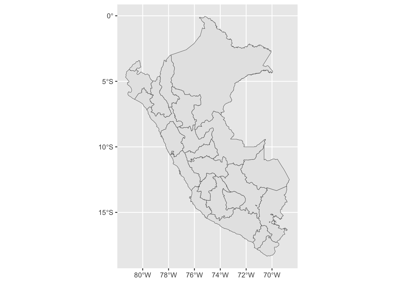
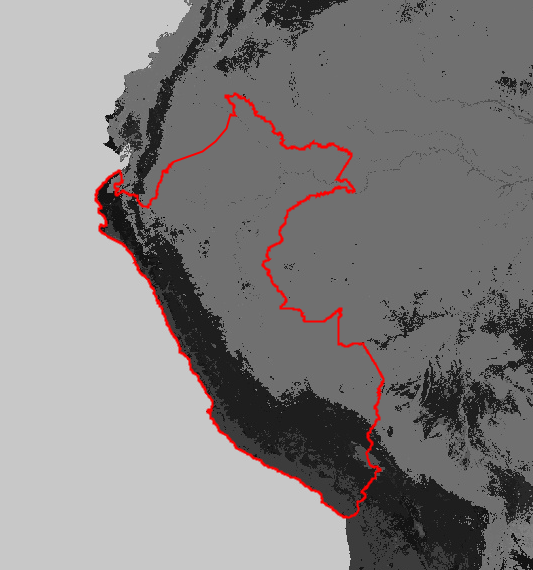
Obtaining a map of Peru: we will explore how to retrieve a map of Peru, providing a visual representation of the geographical area of interest.
Retrieving land use data from Copernicus: this data will provide valuable information about the various land cover types present in Peru.
Importing Weather Data from Gridded data: we will show how to import temperature and precipitation data from NetCDF files.
Create Weather/Climate metrics at the grid cell level.
Aggregate metrics to monthly/quarterly/annual regional level: the metrics defined at the daily grid-cell level will be spatially and temporally aggregated.
A few packages are needed:
library(tidyverse)
── Attaching core tidyverse packages ──────────────────────── tidyverse 2.0.0 ──
✔ dplyr     1.1.4     ✔ readr     2.1.5
✔ forcats   1.0.0     ✔ stringr   1.5.1
✔ ggplot2   3.5.1     ✔ tibble    3.2.1
✔ lubridate 1.9.3     ✔ tidyr     1.3.1
✔ purrr     1.0.2
── Conflicts ────────────────────────────────────────── tidyverse_conflicts() ──
✖ dplyr::filter() masks stats::filter()
✖ dplyr::lag()    masks stats::lag()
ℹ Use the conflicted package (<http://conflicted.r-lib.org/>) to force all conflicts to become errors
# library(rnoaa)library(lubridate)library(sf)
Linking to GEOS 3.11.0, GDAL 3.5.3, PROJ 9.1.0; sf_use_s2() is TRUE
library(rmapshaper)library(raster)
Loading required package: sp

Attaching package: 'raster'

The following object is masked from 'package:dplyr':

    select
As this file is pretty large, we will only focus iteratively on fractions of it. To do so, it is easier to load the TIF file with read_stars() from {stars}.
land <- stars::read_stars("../data/output/land/global_land_cover/raster_land_2015_cropped.tif")
The numerical values associated with each tile of the TIF are the estimated fraction of the 100\(m^2\) covered with agricultural land.
names(land)[1] <-"percent_cropland"
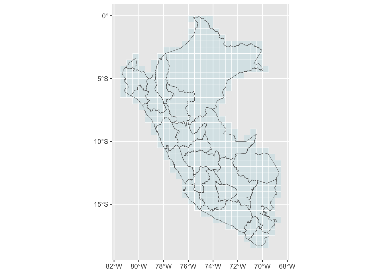
Let us create a function that will consider the ith cell of Peru’s grid (as obtained previously in the Map section). We extract the tiles from the land use raster intersecting with the cell, only keeping tiles within the boundaries. Then, we compute the fraction of cropland. The function returns a table with the value of i, the fraction of cropland, and the area of the cell within the boundaries (in squared metres).
#' Get the cover fractions of cropland for the ith cell of Peru's grid#' #' @param i index of the cell in `map_peru_grid`get_percent_cropland_cell <-function(i) {# Cell from the grid of Peru poly_cell <- map_peru_grid$geometry[i]# Part of that cell within the boundaries poly_cell_in_map <-st_intersection(poly_cell, map_peru) poly_cell_in_map_area <-st_area(poly_cell_in_map) |>sum()# Cropping land cover data land_crop_try <-try(land_crop <-st_crop(land, poly_cell) |>st_as_sf())if (inherits(land_crop_try, "try-error")) { new_bbox_border <-function(bbox){if (bbox[["xmin"]] <st_bbox(land)[["xmin"]]) { bbox[["xmin"]] <-st_bbox(land)[["xmin"]] }if (bbox[["xmax"]] >st_bbox(land)[["xmax"]]) { bbox[["xmax"]] <-st_bbox(land)[["xmax"]] } bbox } new_bbox_poly_cell <-new_bbox_border(st_bbox(poly_cell)) land_crop <-st_crop(land, new_bbox_poly_cell) |>st_as_sf() }# land cover data within the part of the grid cell within the boundaries land_within_cell <-st_intersection(land_crop, poly_cell_in_map)tibble(i = i, percent_cropland =mean(land_within_cell$percent_cropland),area_cell = poly_cell_in_map_area )}
This function just needs to be applied to each cell of the grid. It takes a few hours on a standard 2021 computer.
percent_cropland_cells <-vector(mode ="list", length =nrow(map_peru_grid))pb <-txtProgressBar(min =0, max =nrow(map_peru_grid), style =3)for (i in1:nrow(map_peru_grid)) { percent_cropland_cells[[i]] <-get_percent_cropland_cell(i)setTxtProgressBar(pb, i)}percent_cropland_cells <-bind_rows(percent_cropland_cells)
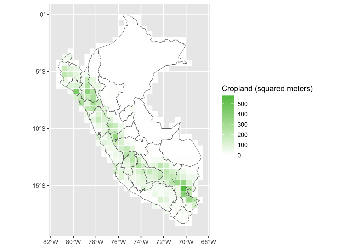
The area of the cell is expressed in squared meters. Let us convert those values to squared kilometres. Then, for each cell, let us compute the cropland area.
While this value makes sense, we get an odd value for the agricultural land. According to the World Bank, agricultural lands correspond to roughly 18% of total land in Peru. We only get 1.7%.
100*sum(map_peru_grid_agri$cropland) /sum(map_peru_grid_agri$area_cell_sqkm) # far from it...
[1] 1.667849
However, what we are interested in here is the relative cropland area. Let us have a look at that.
p <-ggplot() +geom_sf(data = map_peru_grid_agri,mapping =aes(fill = cropland), colour ="white" ) +geom_sf(data = map_peru, fill =NA) +scale_fill_gradient2("Cropland (squared meters)",low ="white", high ="#61C250" )p
Figure 1.4: Agricultural land use in Peru
Even if the values do not add up to 18% of total land, the relative values seem to be close to what can be observed on the Google Earth Engine:
Here is the code used to reproduce that map on Google Earth Engine:
var dataset =ee.Image("COPERNICUS/Landcover/100m/Proba-V-C3/Global/2019").select('discrete_classification');Map.setCenter(-88.6, 26.4, 1);Map.addLayer(dataset, {}, "Land Cover");var worldcountries =ee.FeatureCollection('USDOS/LSIB_SIMPLE/2017');var filterCountry =ee.Filter.eq('country_na', 'Peru');var country =worldcountries.filter(filterCountry);var styling = {color:'red', fillColor:'00000000'};Map.addLayer(country.style(styling));Map.centerObject(country, 5);
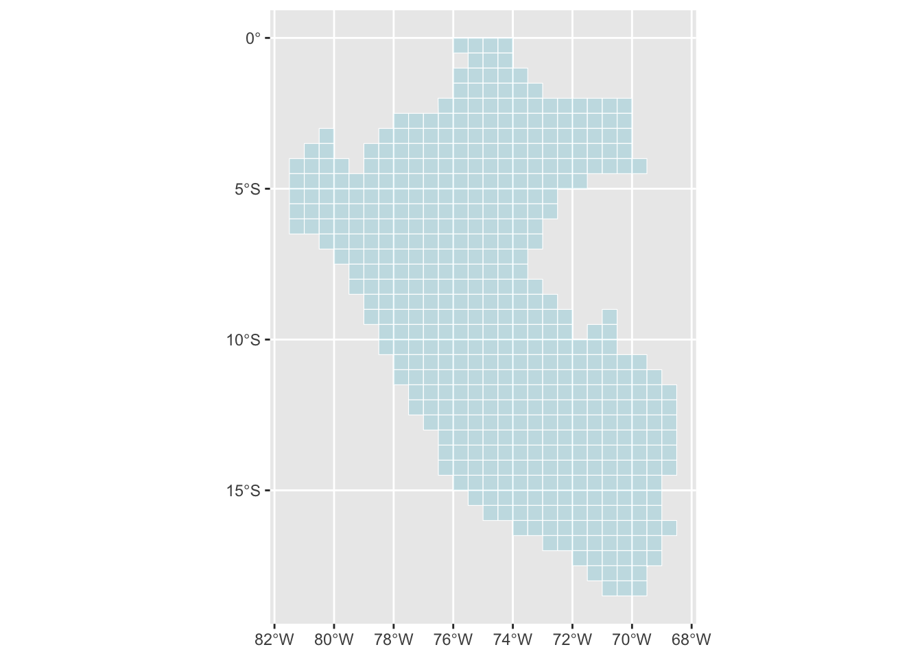
We will loop over the cells of the map of Peru. For each cell, we will load chunks of data iteratively (because the size of the data is too large to be loaded in memory). Let us consider 500 chunks.
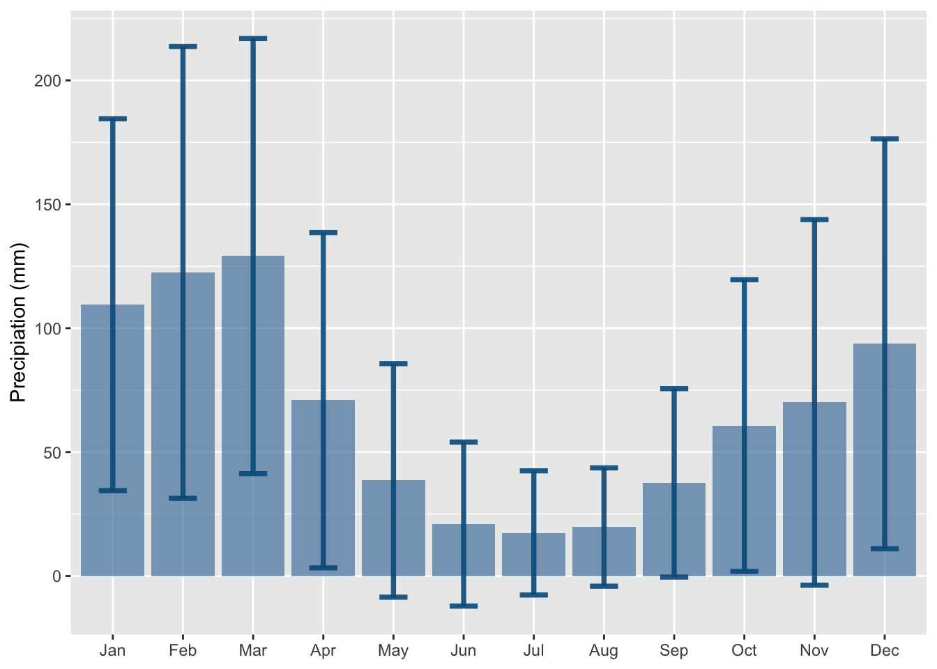
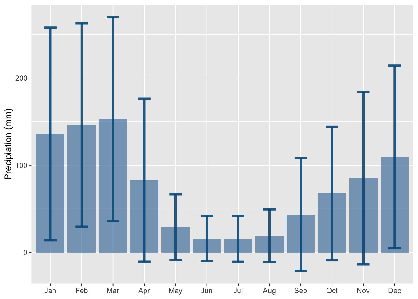
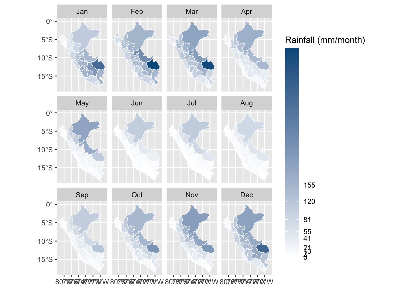
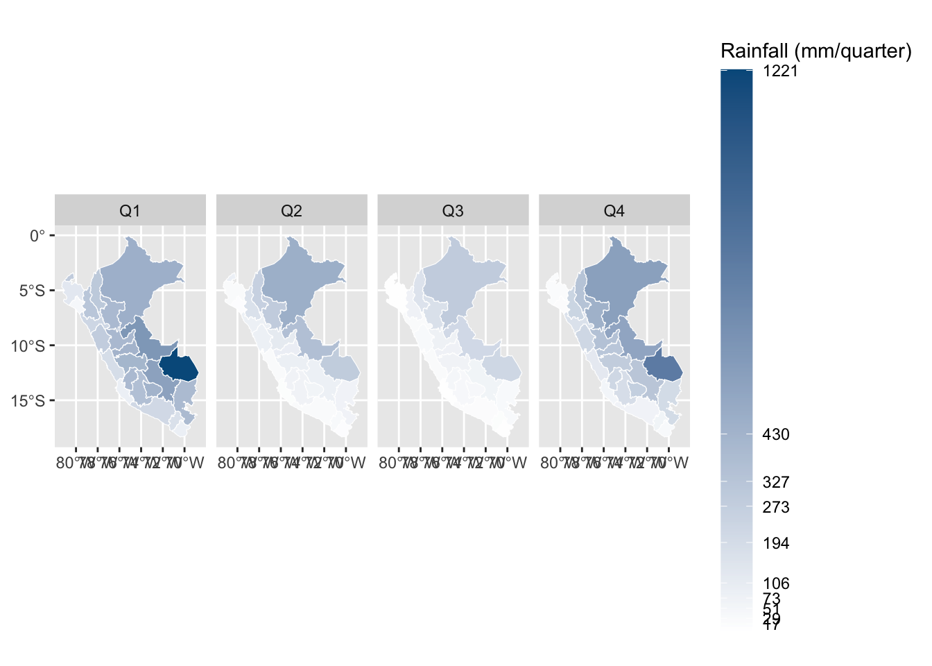
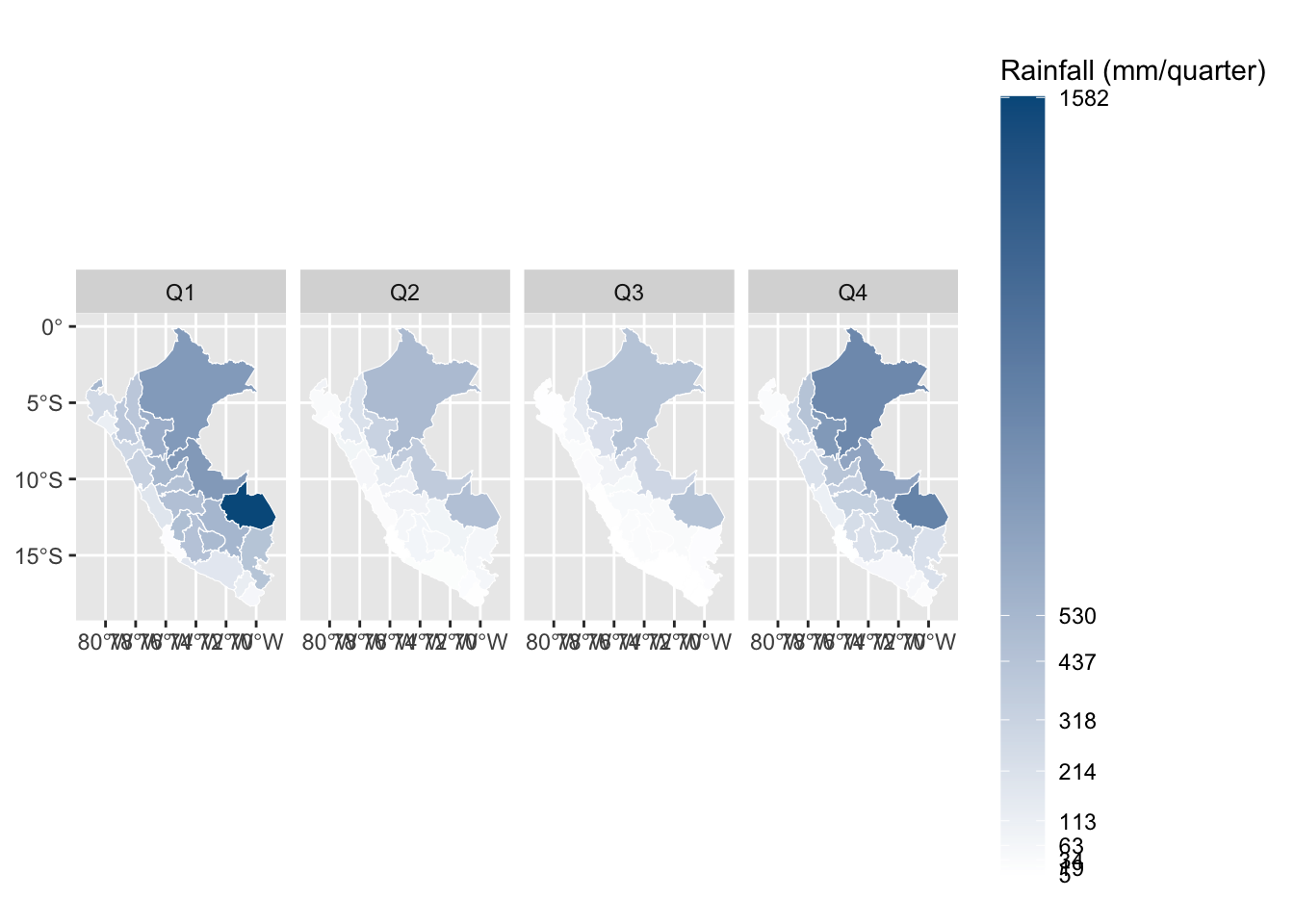
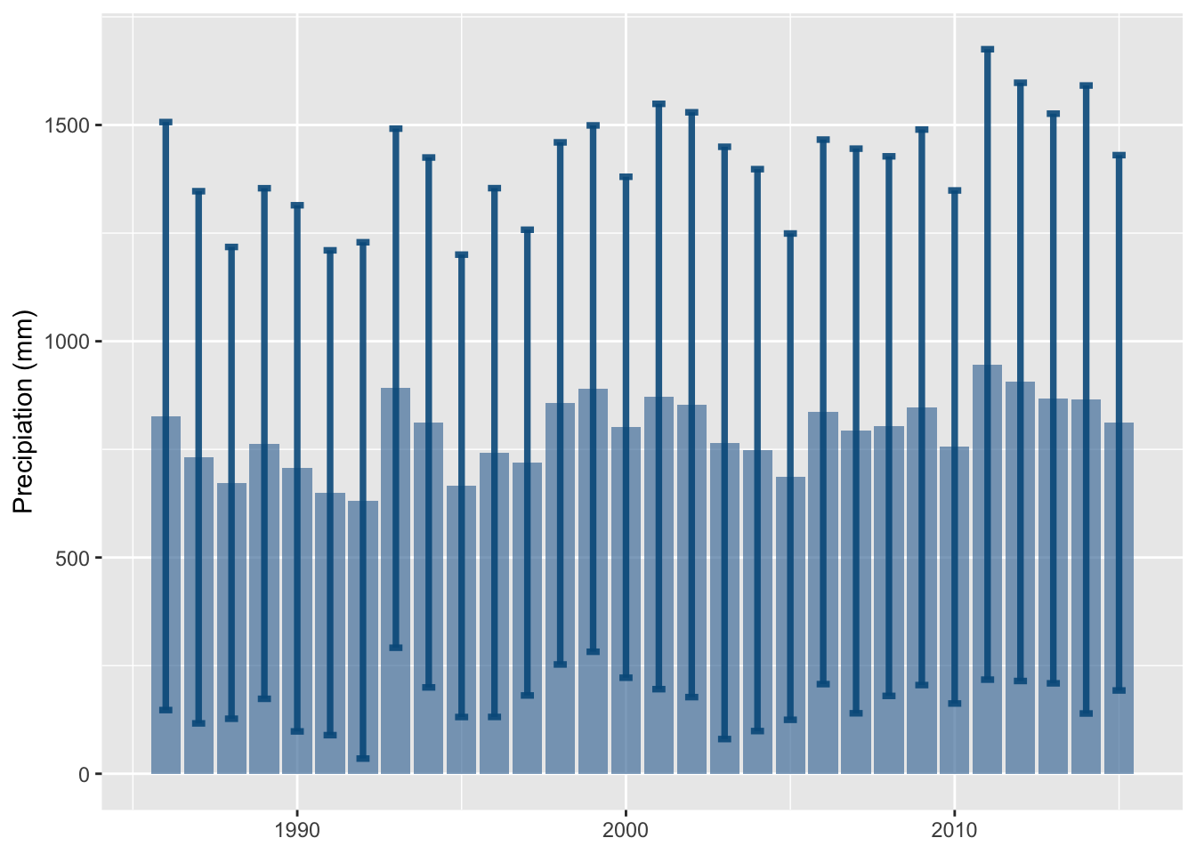
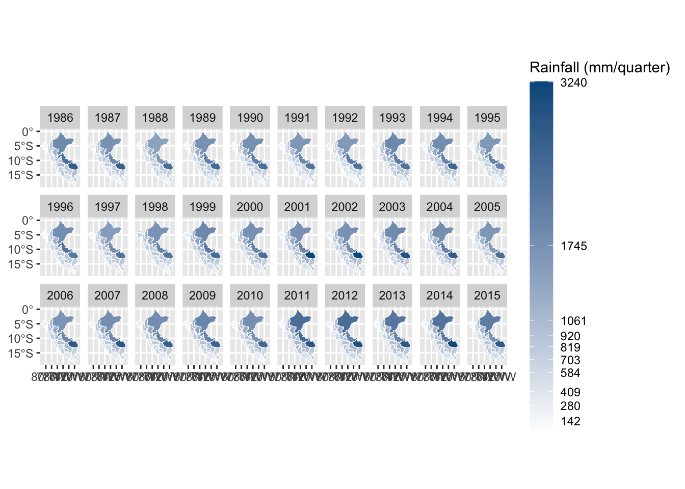
The rainfall data are obtained from the CHIRPS v2.0 database, made available by the Climate Hazards Center of the UC Santa Barbara. Covering the quasi totality of the globe, the data set provides daily information on rainfall on a 0.05° resolution satellite imagery, from 1981 to present. The complete presentation of the data can be found on the Climate Hazards Center’s website Funk et al. (2015) and the data set is freely available online.
N <-list.files("data/raw/weather/CHIRPS-2_0_global_daily_p25", pattern ="\\.nc$", full.names =TRUE)
Let us loop over the files (one per year). At each iteration, let us save the intermediate results.
for (ii in1:length(N)) { file <- N[ii] precip_sf_raster <- raster::raster(file)proj4string(precip_sf_raster) <-CRS("+init=EPSG:4326") precip_sf <- stars::st_as_stars(precip_sf_raster) |> sf::st_as_sf() sf::sf_use_s2(FALSE) precip_sf$geometry <- precip_sf$geometry |> s2::s2_rebuild() |> sf::st_as_sfc() precip_grille_i <-vector(mode ="list", length =nrow(map_peru_grid)) pb <-txtProgressBar(min=0, max=nrow(map_peru_grid), style=3)for (k in1:nrow(map_peru_grid)) {# Average precipitations in the k-th cell tmp <-suppressMessages(st_interpolate_aw(precip_sf, map_peru_grid[k,], extensive =FALSE) )# Each column of `tmp` gives the average for a given date tmp <-tibble(tmp)# Let us transform `tmp` so that each row gives the average precipitations # in the k-th cell, for a specific date tmp_2 <- tmp |> tidyr::pivot_longer(cols =-c(geometry), names_to ="date_v") |> dplyr::mutate(date =str_remove(date_v, "^X") |> lubridate::ymd()) |> dplyr::select(-date_v, -geometry) |> dplyr::mutate(grid_id = k)# Add the ID of the k-th cell precip_grille_i[[k]] <- tmp_2setTxtProgressBar(pb, k) } precip_grille <- precip_grille_i |>bind_rows() file_name <-str_replace(file, "\\.nc$", ".rda") file_name <-str_replace(file_name, "data/raw/", "data/output/")save(precip_grille, file = file_name)}
The intermediate results can be loaded again, and merged to a single tibble:
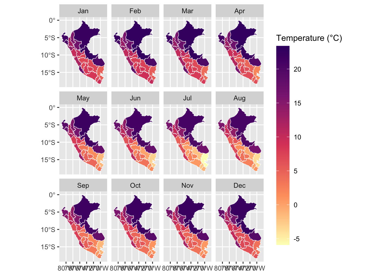
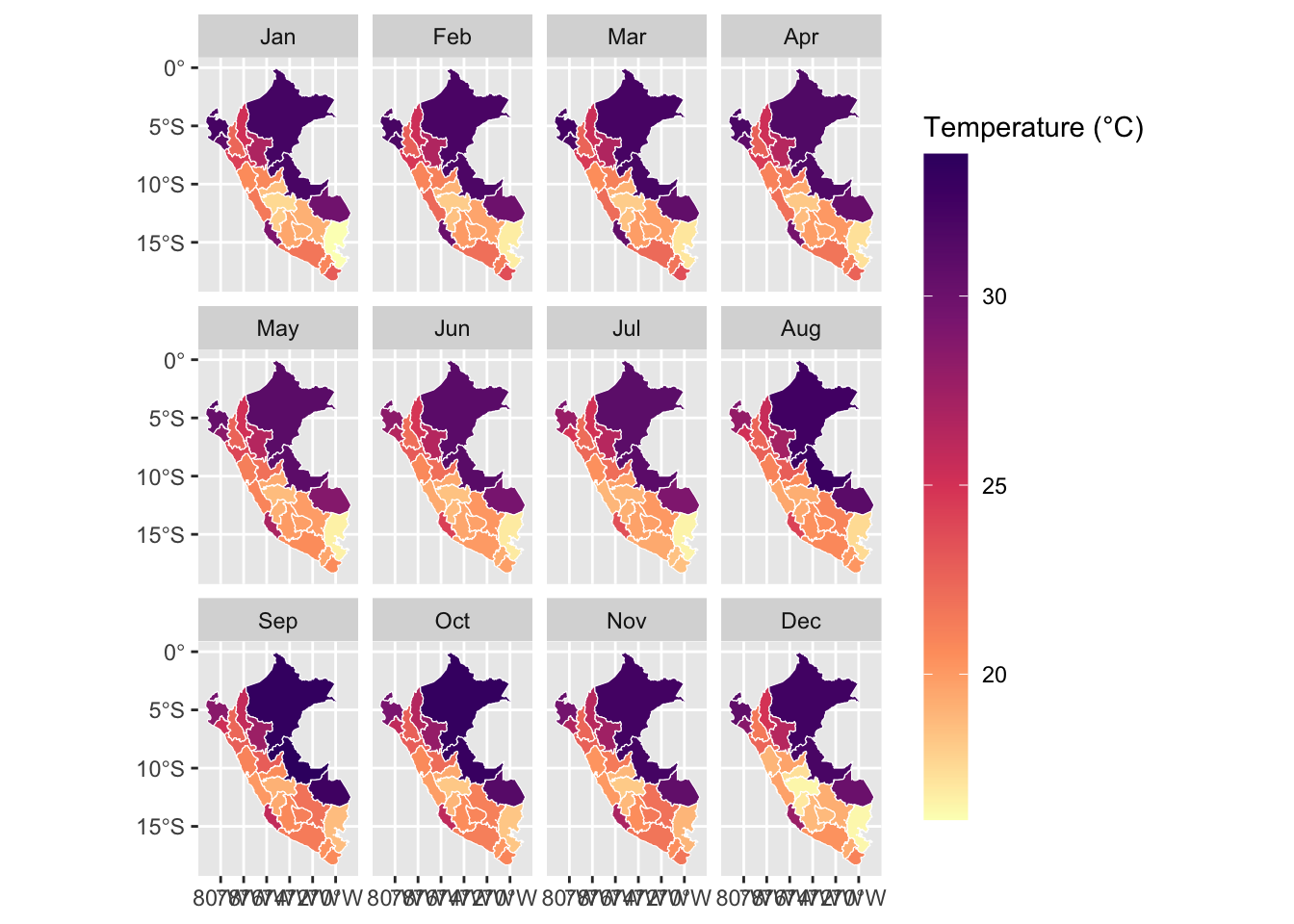
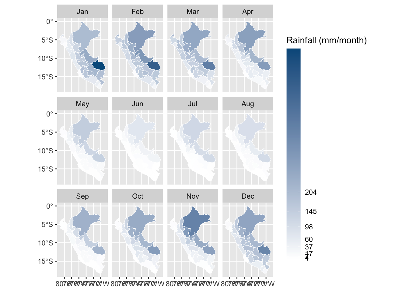
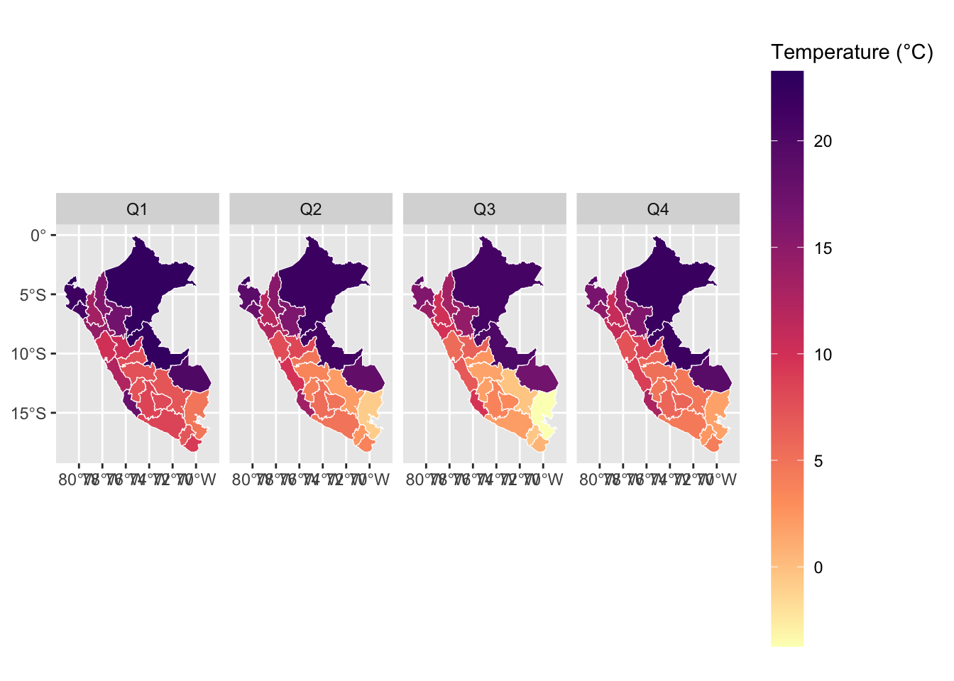
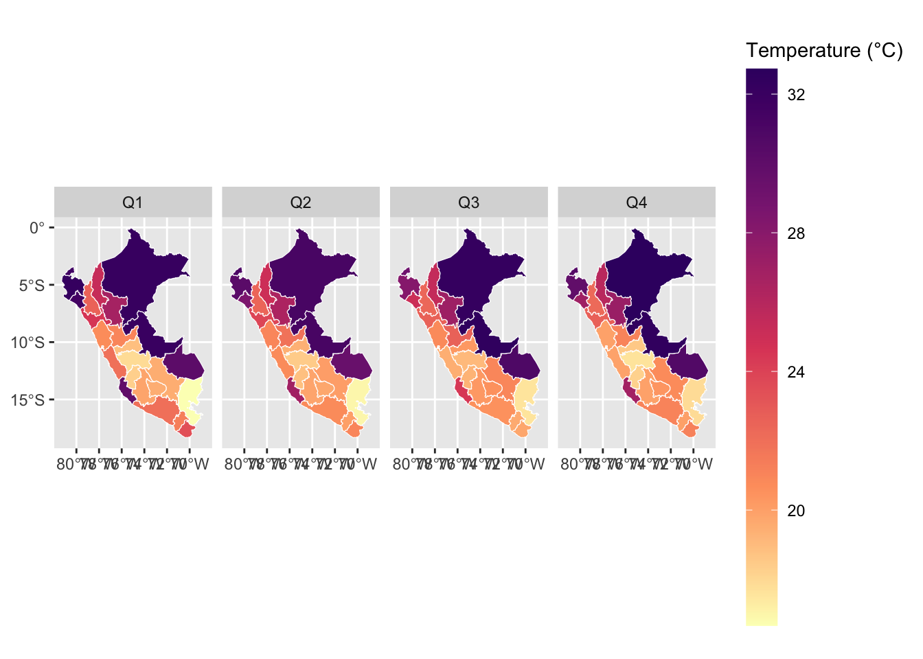
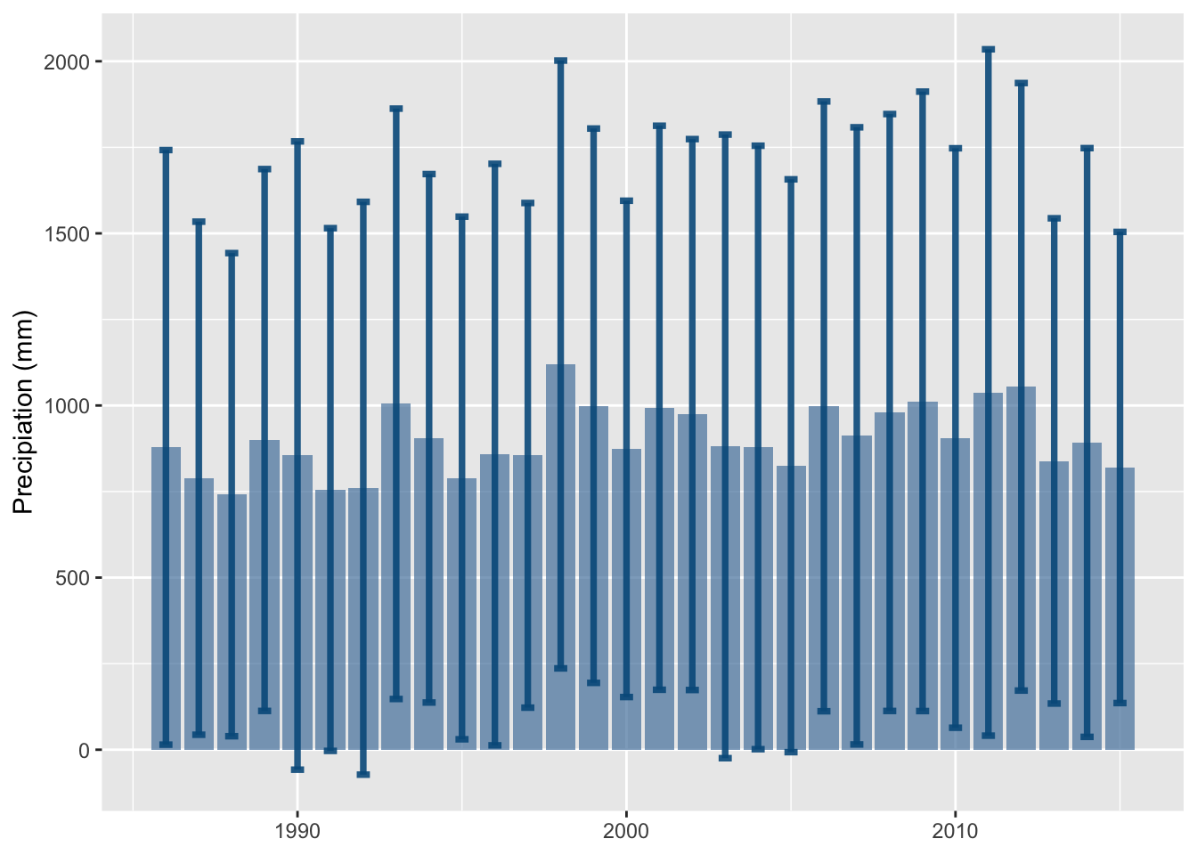
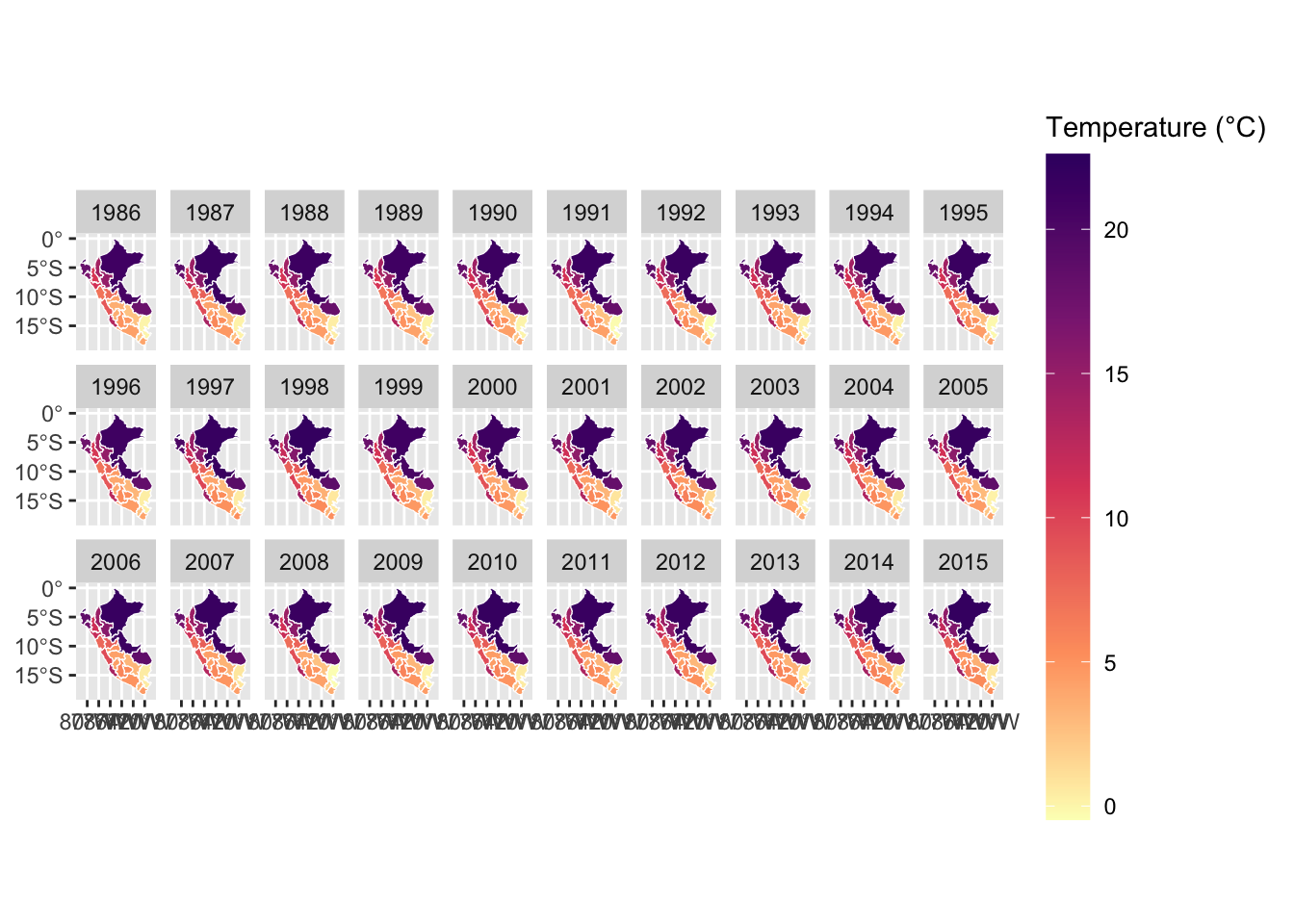
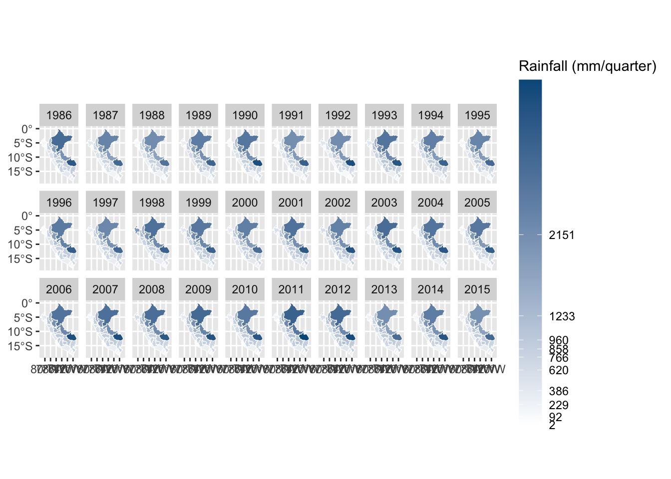
We use the PISCO temperature dataset version 1.1c (PISCOt). The PISCOt dataset represents a gridded product of maximum (tx) temperature and minimum (tn) temperature at a spatial resolution of 0.1° for Peru. It is available at daily (d), monthly (m), and annual (a) scales. In this analysis, we utilize the daily values of the PISCOt dataset. More details can be found on Github.
1.3.3.1 Minimum Temperatures
First, we load the raster data corresponding to the daily minimum temperatures:
We will loop over the cells of the map of Peru. For each cell, we will load chunks of data iteratively (because the size of the data is too large to be loaded in memory). Let us consider 500 chunks.
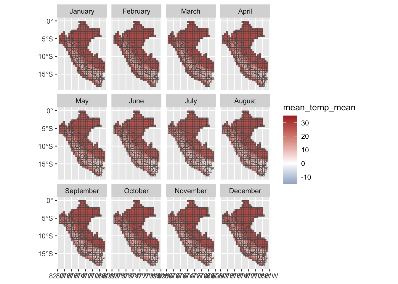
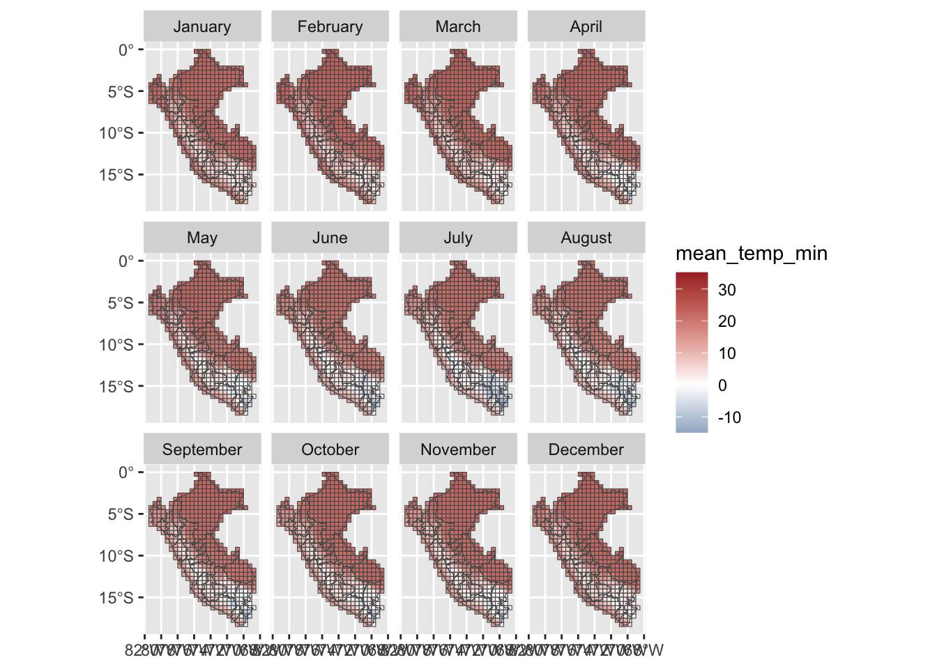
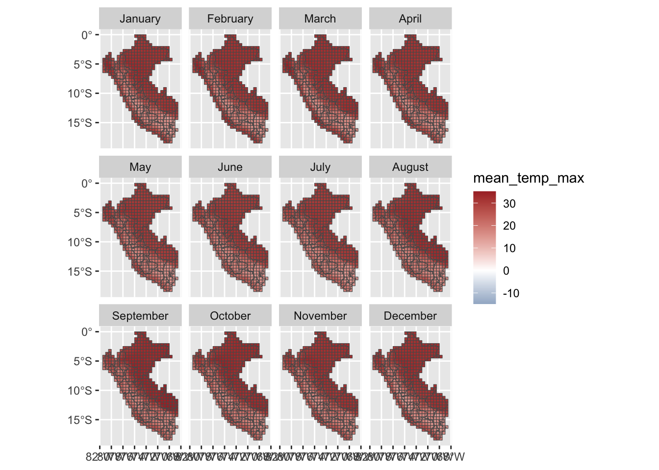
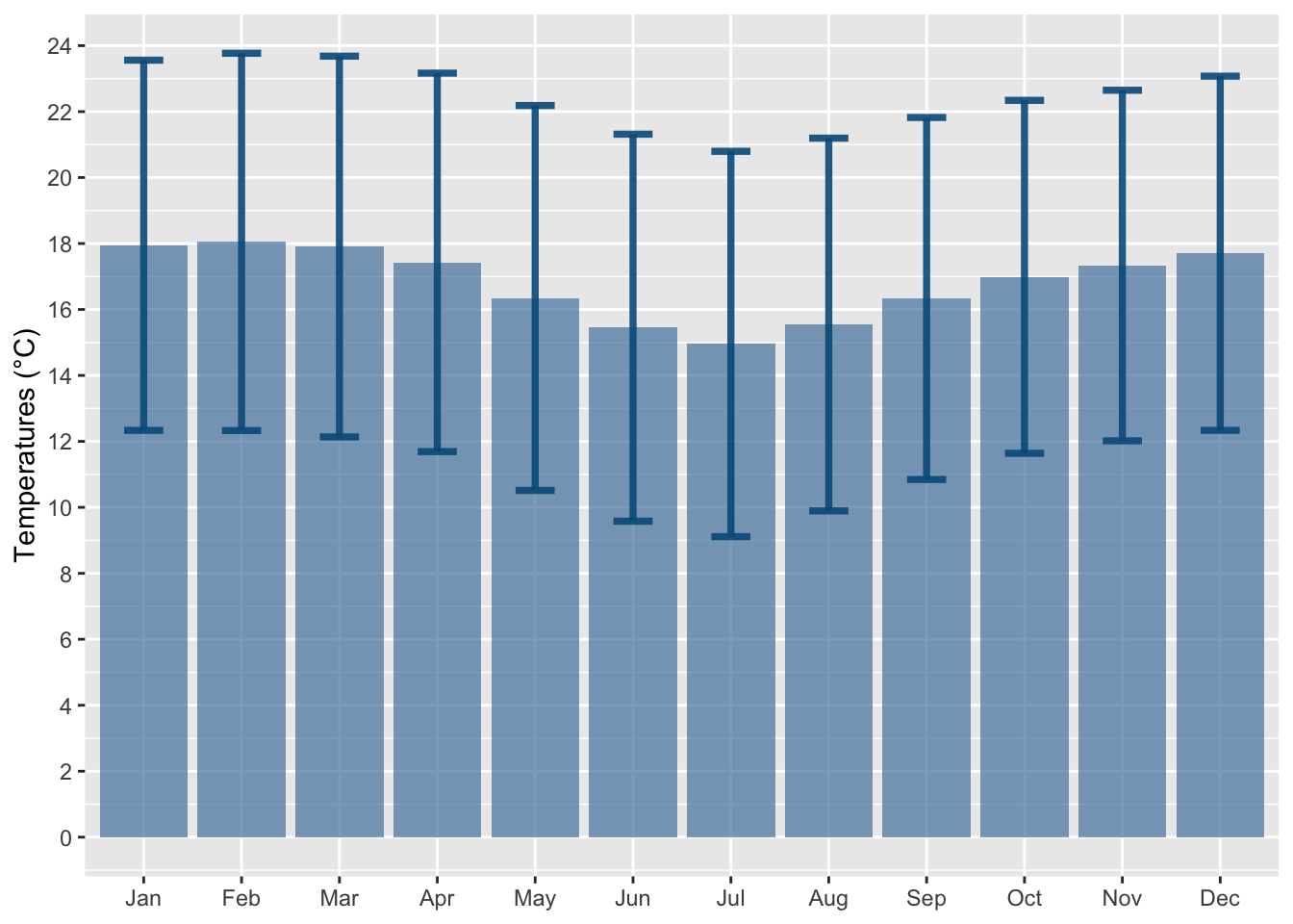
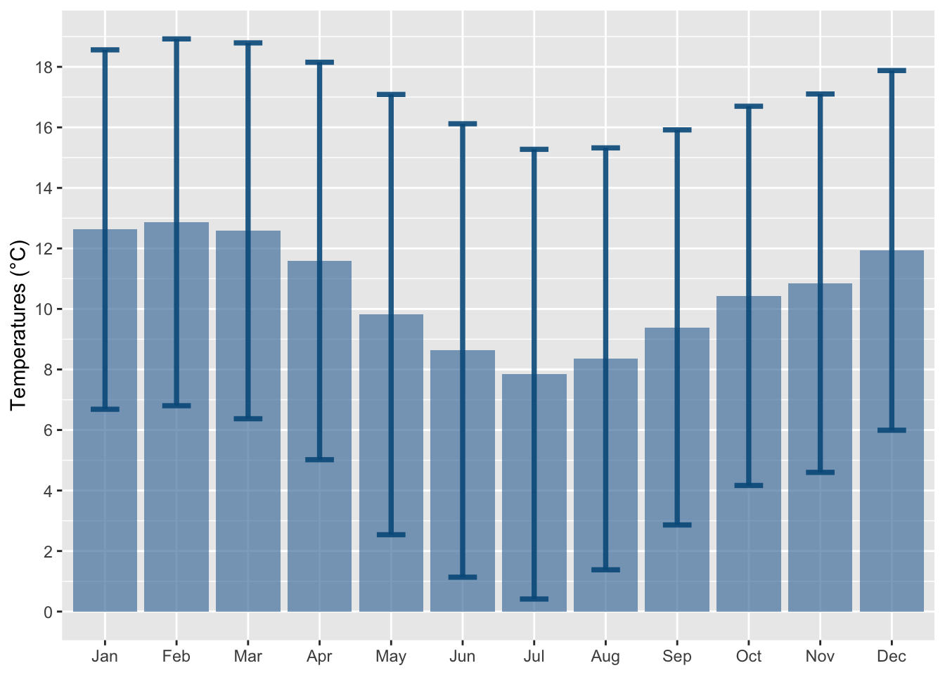
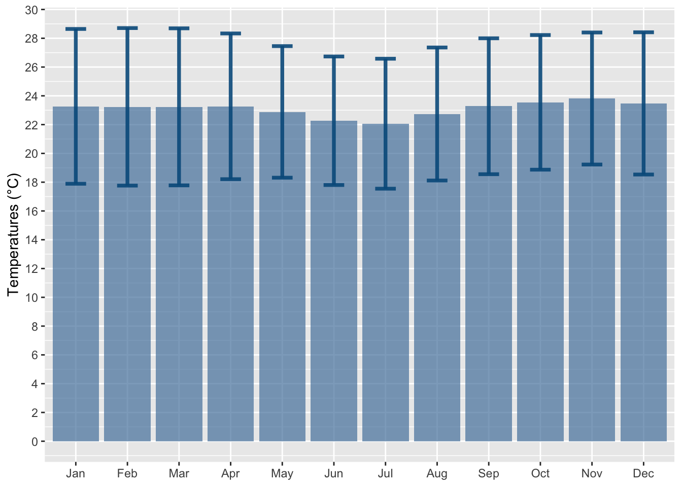
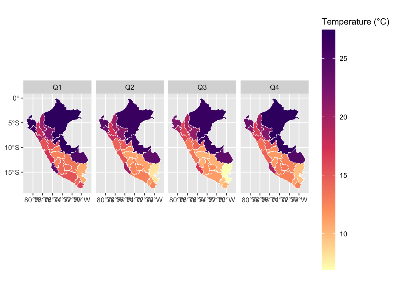
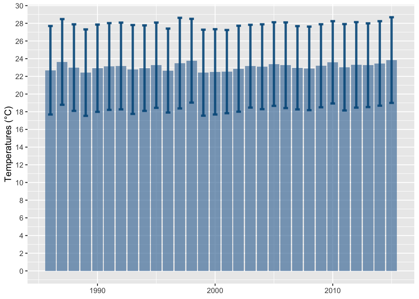
Let us visualize the data at the grid level. We only look at the example of 2010. We compute the monthly average of daily mean, min, and maximum temperatures.
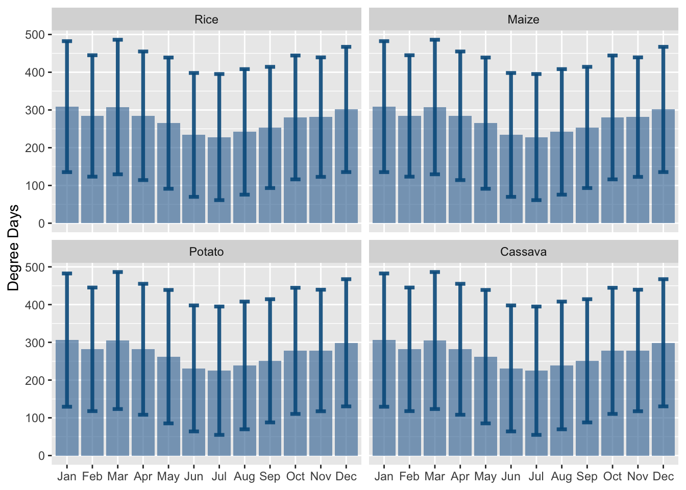
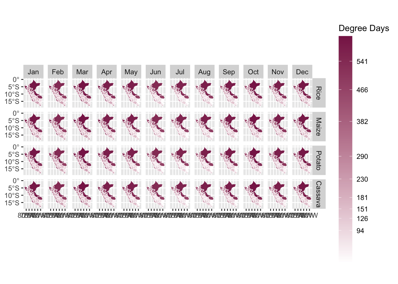
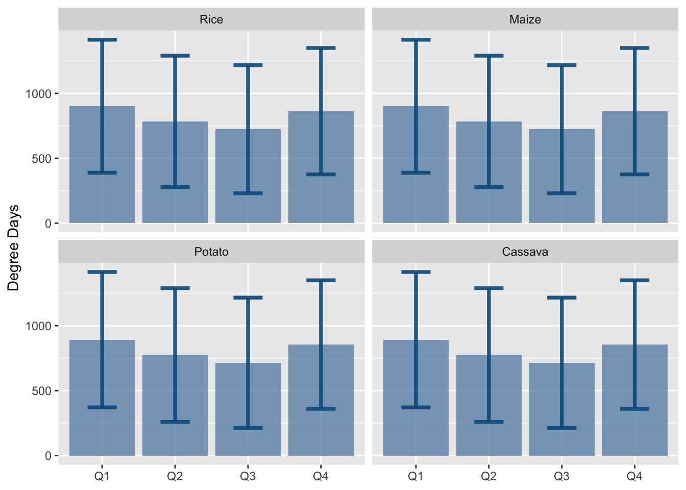
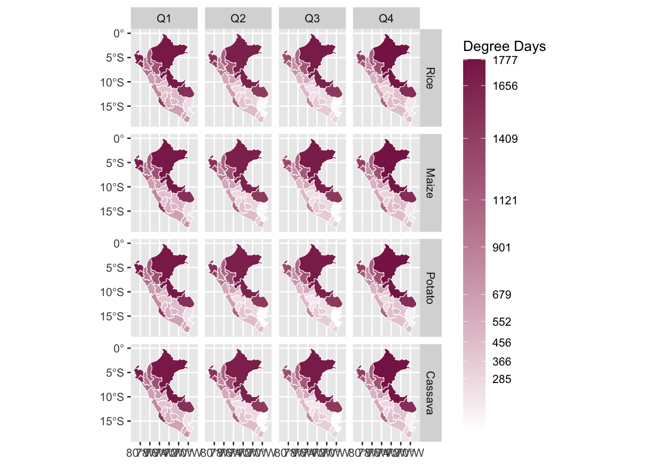
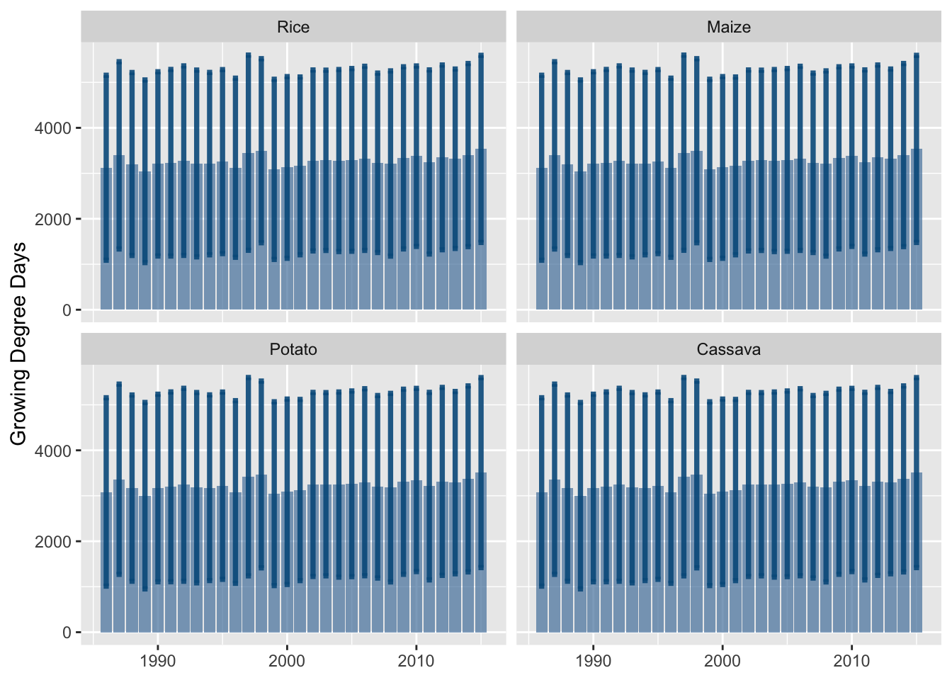
Following Aragón, Oteiza, and Rud (2021), we compute degree days, with crop-specific threshold values. \[
\text{DD} = \frac{1}{n} \sum_{d=1}^{n}\left(\min{(h_d, \tau)} - \tau_{\ell}\right) \mathbf{1}(h_d\geq 8),
\] where \(h_d\) is the average observed temperature observed in day \(d\), \(n\) is the number of days in the period of interest (month, quarter, or year), \(\tau\) is a crop-specific threshold set to 29 for rice and maize and set to 30 for potato and cassava. The parameter \(\tau_{\ell}\) is a lower bound set to 8 for all crops.
Degree days capture the cumulative exposure to temperatures comprised between the lower bound \(\tau_{\ell}\) and the upper bound \(\tau\).
# Degree Daysweather_peru_daily_grid <- weather_peru_daily_grid |>mutate(gdd_daily_rice = temp_mean -8,gdd_daily_rice =ifelse(temp_mean >29, yes =21, no = gdd_daily_rice),gdd_daily_rice =ifelse(temp_mean <8, yes =0, no = gdd_daily_rice),#gdd_daily_maize = temp_mean -8,gdd_daily_maize =ifelse(temp_mean >29, yes =21, no = gdd_daily_maize),gdd_daily_maize =ifelse(temp_mean <8, yes =0, no = gdd_daily_maize),#gdd_daily_potato = temp_mean -10,gdd_daily_potato =ifelse(temp_mean >30, yes =20, no = gdd_daily_potato),gdd_daily_potato =ifelse(temp_mean <10, yes =0, no = gdd_daily_potato),#gdd_daily_cassava = temp_mean -10,gdd_daily_cassava =ifelse(temp_mean >30, yes =20, no = gdd_daily_cassava),gdd_daily_cassava =ifelse(temp_mean <10, yes =0, no = gdd_daily_cassava) )
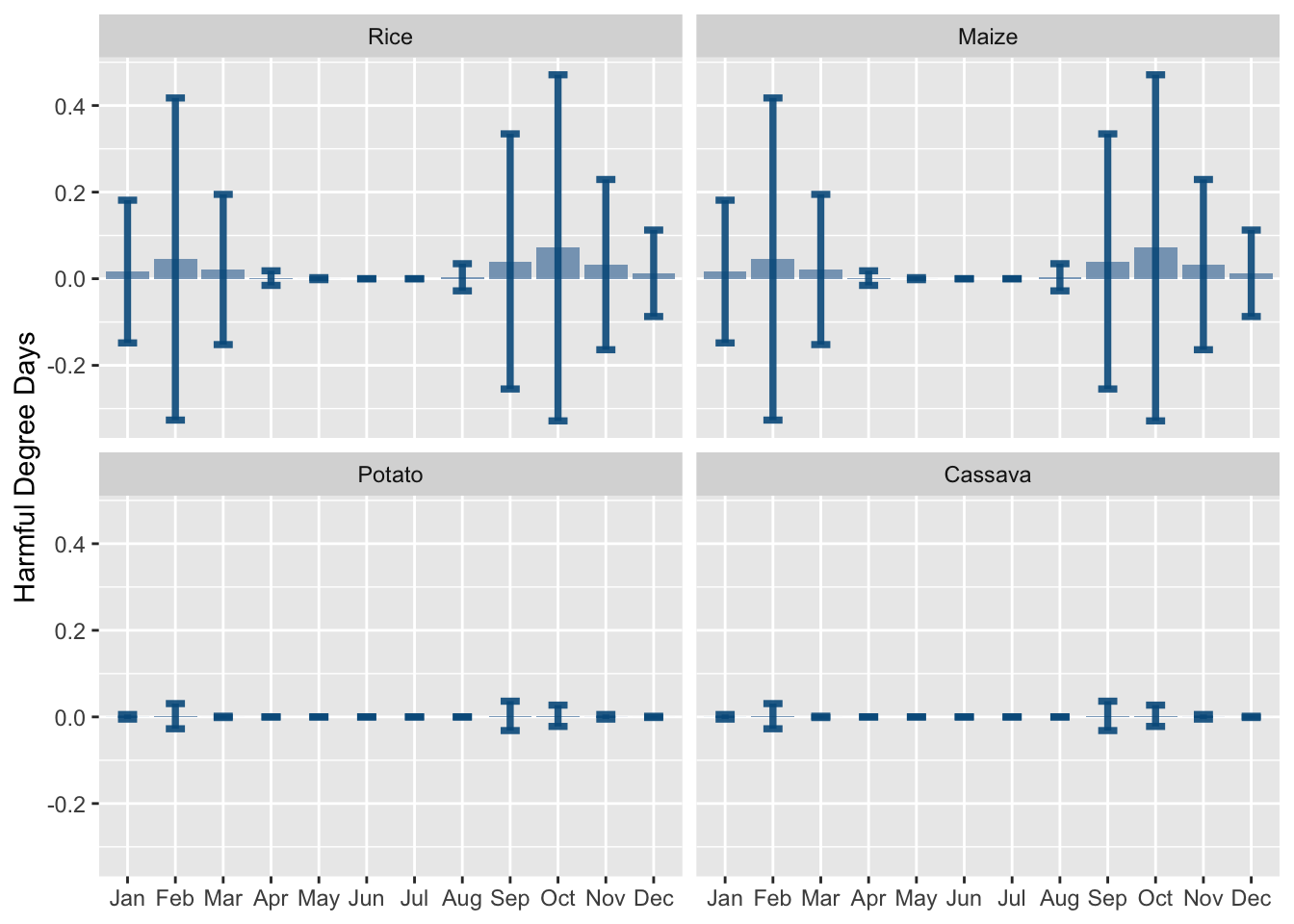
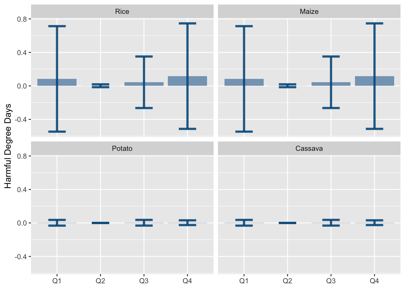
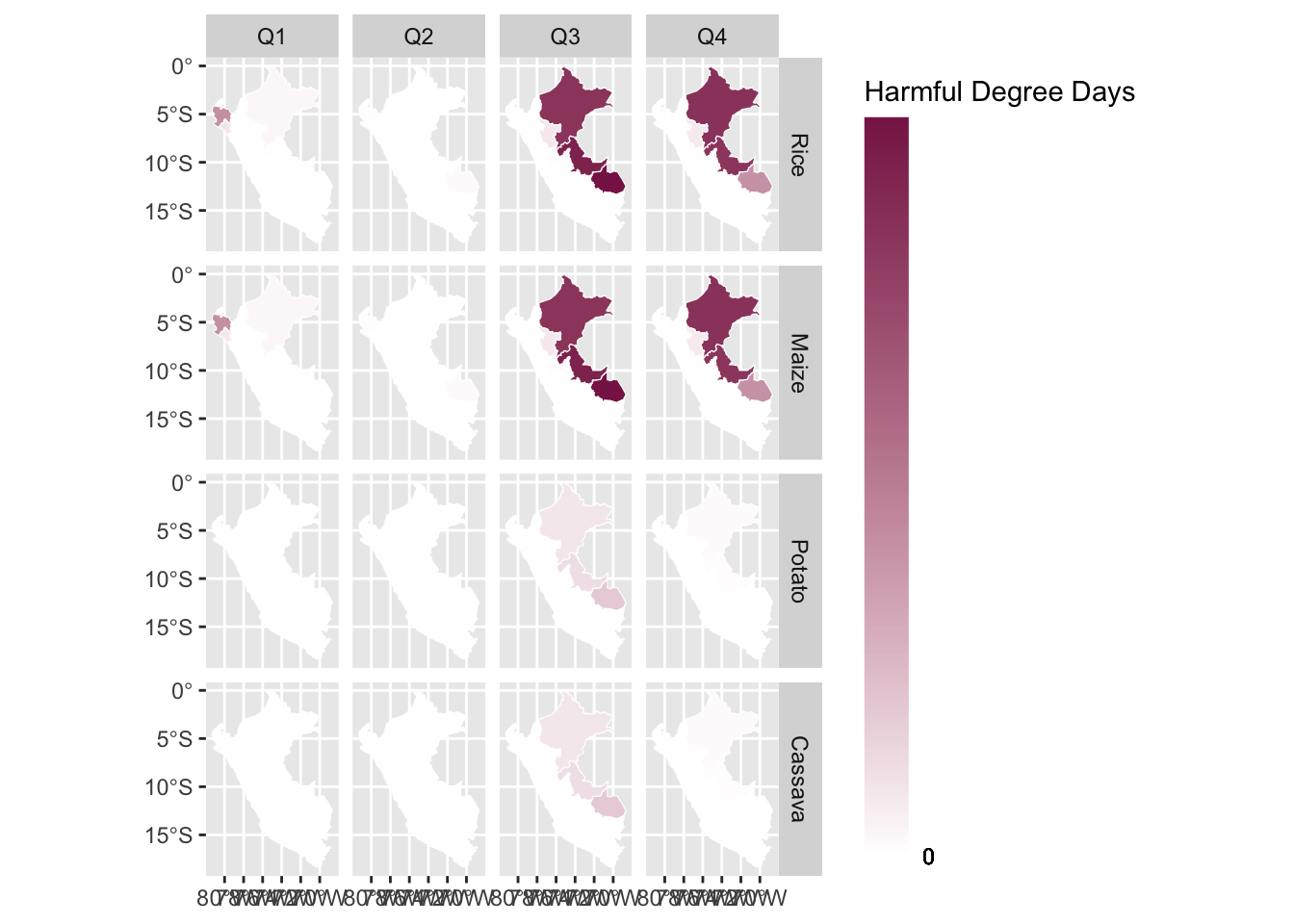
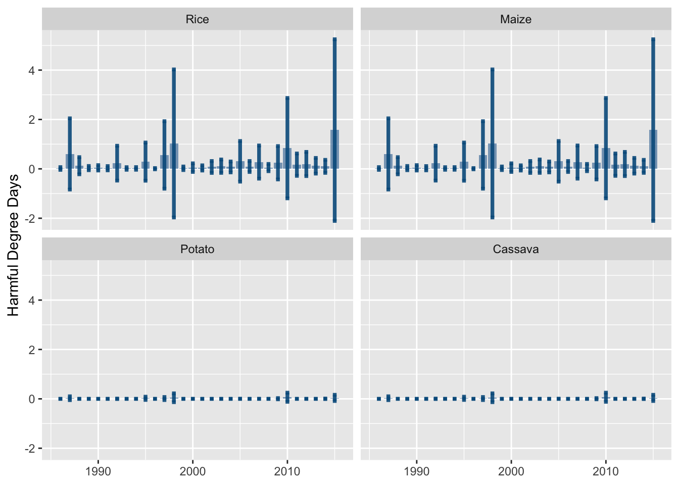
1.4.2 Harmful Degree Days
We also define harmful degree days (Aragón, Oteiza, and Rud (2021)): \[
\text{HDD} = \frac{1}{n}\sum_{d=1}^{n} = \left(h_d - \tau_{\text{high}}\right) \mathbf{1}(h_d > \tau_\ell),
\] where \(\tau_{\text{high}}\) is a crop-specific threshold set to 29 for rice and maize and set to 30 for potato and cassava.
weather_peru_daily_grid <- weather_peru_daily_grid |>mutate(hdd_daily_maize =ifelse(temp_mean >29, yes = temp_mean -29, no =0), hdd_daily_rice =ifelse(temp_mean >29, yes = temp_mean -29, no =0), hdd_daily_potato =ifelse(temp_mean >30, yes = temp_mean -30, no =0), hdd_daily_cassava =ifelse(temp_mean >30, yes = temp_mean -30, no =0) )
1.4.3 Cold / Hot / Dry / Wet Surprise Days
We follow Natoli (2024) and define cold and hot surprise weather shocks.
The idea is to compare the realized temperatures that occurred during a month \(m\) of a year \(y\) in a location \(c\) with the expected realizations calculated from the past observed temperatures during the same month \(m\) in previous years at the same location \(c\). The difference between these two values is defined as a surprise shock.
The shock in cell \(c\) is defined as follows for days hotter than expected during month \(m\) of year \(y\): \[
\mathcal{W}\text{hot}_{c,y,m} = \underbrace{\sum_{d=1}^{n_{m}} \mathrm{1}\left(\mathcal{T}_{c,y,m,d} > \text{ut}_{c,y,m} \right)}_{\text{observed realizations}} - \underbrace{\frac{1}{5}\sum_{k=1}^{5}\sum_{d=1}^{n_m} \mathrm{1}\left(\mathcal{T}_{c,y-k,m,d} > \text{ut}_{c,y,m}\right)}_{\text{expected realizations}},
\tag{1.1}\]
where \(\mathcal{T}_{c,y,m,d}\) is the average temperature observed on day \(d\) of month \(m\) in year \(y\) in cell \(c\), \(n_m\) is the number of days in month \(m\), and \(\text{ut}_{c,y,m}\) is a threshold above which the daily average temperature is considered hot.
Similarly, surprise cold shocks are defined as follows: \[
\mathcal{W}\text{cold}_{c,y,m} = \underbrace{\sum_{d=1}^{n_{m}} \mathrm{1}\left(\mathcal{T}_{c,y,m,d} < \text{lt}_{c,y,m} \right)}_{\text{observed realizations}} - \underbrace{\frac{1}{5}\sum_{k=1}^{5}\sum_{d=1}^{n_m} \mathrm{1}\left(\mathcal{T}_{c,y-k,m,d} < \text{lt}_{c,y,m}\right)}_{\text{expected realizations}},
\tag{1.2}\]
where \(\text{lt}_{c,y,m}\) is a threshold used to define cold days.
The thresholds \(\text{ut}_{c,y,m}\) and \(\text{lt}_{c,y,m}\) are defined using the average temperature observations during month \(m\) of the 5 years preceding year \(y\), denoted as \(\boldsymbol{T}_{c,y,d} = \left\{\{\mathcal{T}_{c,y-1,m,d}\}_{d=1}^{n_m}, \{\mathcal{T}_{c,y-2,m,d}\}_{d=1}^{n_m}, \ldots, \{\mathcal{T}_{c,y-5,m,d}\}_{d=1}^{n_m}\}\right\}\). Based on the observations \(\boldsymbol{T}_{c,y,d}\), the empirical 10th and 90th percentiles are calculated, \(P_{10}(\boldsymbol{T}_{c,y,d})\) and \(P_{90}(\boldsymbol{T}_{c,y,d})\).
In Natoli (2024), the thresholds are constructed as follows: \[
\begin{align}
\text{ut}_{c,y,m} &= \max\left\{P_{90}(\boldsymbol{T}_{c,y,d}), \tau_{\text{upper}}\right\}\\
\text{lt}_{c,y,m} &= \min\left\{P_{10}(\boldsymbol{T}_{c,y,d}), \tau_{\text{lower}}\right\}
\end{align}
\] where \(\tau_{\text{upper}}\) and \(\tau_{\text{lower}}\) are arbitrarily fixed values. Here, we rely on agronomic literature to choose the values: \(\tau_{\text{upper}} = 29^\circ\)C for rice and maize, and \(\tau_{\text{upper}} = 30^\circ\)C for potatoes and cassava. For \(\tau_{\text{lower}}\), we set the value at \(8^\circ\)C for rice and maize, and \(10^\circ\)C for potatoes and cassava.
Similarly, we define surprise precipitation shocks for dry days as follows: \[
\mathcal{W}\text{dry}_{c,y,m} = \underbrace{\sum_{d=1}^{n_{m}} \mathrm{1}\left(\mathcal{P}_{c,y,m,d} < \text{lt}_{c,y,m} \right)}_{\text{observed realizations}} - \underbrace{\frac{1}{5}\sum_{k=1}^{5}\sum_{d=1}^{n_m} \mathrm{1}\left(\mathcal{P}_{c,y-k,m,d} < \text{lt}_{c,y,m}\right)}_{\text{expected realizations}},
\tag{1.3}\]
where \(\mathcal{P}_{c,y,m,d}\) represents total precipitation. And for wet days:
In the case of dry/wet days, the thresholds are simply defined using percentiles: \[
\begin{cases}
\text{ut}_{c,y,m} & = P_{90}(\boldsymbol{P}_{c,y,d})\\
\text{lt}_{c,y,m} & = P_{10}(\boldsymbol{P}_{c,y,d})
\end{cases}
\] with \(\boldsymbol{P}_{c,y,d} = \left\{\{\mathcal{P}_{c,y-1,m,d}\}_{d=1}^{n_m}, \{\mathcal{P}_{c,y-2,m,d}\}_{d=1}^{n_m}, \ldots, \{\mathcal{P}_{c,y-5,m,d}\}_{d=1}^{n_m}\}\right\}\) representing the total daily precipitation observed during month \(m\) in the 5 years preceding year \(y\) in cell \(c\).
Let us implement this in R. First, let us extract the year and month of each observation from the grid.
Then, we define function get_surprise_w_shocks_monthly() that computes, for a specific month \(m\) in year \(y\) the surprise shocks for each cell.
#' Computes the cell-level cold surprise and hot surprise with respect to the #' daily temperatures in the past years#' # Natoli, Filippo, The Macroeconomic Effects of Unexpected Temperature Shocks # (April 11, 2024). # Available at SSRN: https://ssrn.com/abstract=4160944#' #' @paam year year to consider#' @param month month to consider#' @param window number of years for the window#' @param upper_threshold upper threshold above which a day is considered hot#' @param lower_threshold upper threshold above which a day is considered coldget_surprise_w_shocks_monthly <-function(year, month, window, upper_threshold, lower_threshold) {# Focus on values from the previous `window` years for the same month years_window <-seq(year-window, year-1) weather_window <- weather_peru_daily_grid |>filter(year %in%!!years_window, month ==!!month)# Compute 10th and 90th percentiles of daily temperatures for each cell over# the past years# Then compute the expected number of cold/hot days in each cell# (as the average of the number of cold/hot days observed over the window, # in each cell) weather_expected <- weather_window |>nest(.by = grid_id) |>mutate(p10_temp =map(data, ~quantile(.x$temp_mean, probs = .1, na.rm =TRUE)),p90_temp =map(data, ~quantile(.x$temp_mean, probs = .9, na.rm =TRUE)),p10_precip_piscop =map( data, ~quantile(.x$precip_piscop, probs = .1, na.rm =TRUE) ),p90_precip_piscop =map( data, ~quantile(.x$precip_piscop, probs = .9, na.rm =TRUE) ) ) |>unnest(cols =c( data, p10_temp, p90_temp, p10_precip_piscop, p90_precip_piscop) ) |> dplyr::select( grid_id, date, year, month, p10_temp, p90_temp, p10_precip_piscop, p90_precip_piscop, temp_mean, precip_piscop ) |>mutate(lt_temp =pmin(p10_temp, lower_threshold, na.rm =TRUE),ut_temp =pmax(p90_temp, upper_threshold, na.rm =TRUE),lt_precip_piscop = p10_precip_piscop,ut_precip_piscop = p90_precip_piscop ) |>mutate(is_cold = temp_mean < lt_temp,is_hot = temp_mean > ut_temp,is_dry = precip_piscop < lt_precip_piscop,is_wet = precip_piscop > ut_precip_piscop ) |># Number of cold/hot days in the month of each cell, for each yeargroup_by( grid_id, year, month, lt_temp, ut_temp, lt_precip_piscop, ut_precip_piscop ) |>summarise(nb_cold_expected =sum(is_cold, na.rm =TRUE),nb_hot_expected =sum(is_hot, na.rm =TRUE),nb_dry_expected =sum(is_dry, na.rm =TRUE),nb_wet_expected =sum(is_wet, na.rm =TRUE),.groups ="drop" ) |># Average number of cold/hot days in each cell, over the windowgroup_by( grid_id, month, lt_temp, ut_temp, lt_precip_piscop, ut_precip_piscop ) |>summarise(nb_cold_expected =mean(nb_cold_expected, na.rm =TRUE),nb_hot_expected =mean(nb_hot_expected, na.rm =TRUE),nb_dry_expected =mean(nb_dry_expected, na.rm =TRUE),nb_wet_expected =mean(nb_wet_expected, na.rm =TRUE),.groups ="drop" )# The weather data for the current (year, month), for all cells weather_current <- weather_peru_daily_grid |>filter(year ==!!year, month ==!!month) weather_current |> dplyr::select(date, grid_id, temp_mean, precip_piscop, year, month) |>left_join(weather_expected, by =c("grid_id", "month")) |>mutate(is_cold = temp_mean < lt_temp,is_hot = temp_mean > ut_temp,is_dry = temp_mean < lt_precip_piscop,is_wet = temp_mean > ut_precip_piscop ) |>group_by( year, month, grid_id, nb_cold_expected, nb_hot_expected, nb_dry_expected, nb_wet_expected ) |>summarise(nb_cold_obs =sum(is_cold, na.rm =TRUE),nb_hot_obs =sum(is_hot, na.rm =TRUE),nb_dry_obs =sum(is_dry, na.rm =TRUE),nb_wet_obs =sum(is_wet, na.rm =TRUE),.groups ="drop" ) |>mutate(cold_surprise = nb_cold_obs - nb_cold_expected,hot_surprise = nb_hot_obs - nb_hot_expected,dry_surprise = nb_dry_obs - nb_dry_expected,wet_surprise = nb_wet_obs - nb_wet_expected ) |> dplyr::select( year, month, grid_id, cold_surprise, hot_surprise, dry_surprise, wet_surprise )}
Since the get_surprise_w_shocks_monthly() function returns the surprise shocks for a single month of a year (but for all cells of the grid), we need to loop over the different months/years of the sample.
The sliding window size is set to 5 (years).
# Five years windowwindow <-5
We prepare a table with the values of the different months/years to consider.
To convert the daily grid data into monthly data, we aggregate the values on a monthly basis while preserving the spatial scale of the grid cells. This allows us to analyze the data at a monthly resolution and maintain consistency with the original grid structure.
Note that we only keep data from 1986 to 2015.
monthly_weather_data <- weather_peru_daily_grid |>mutate(# year = lubridate::year(date),# month = lubridate::month(date),month_name = lubridate::month( date, abbr =FALSE, label =TRUE, locale ="en_US" ) ) |># Keeping 30 years of datafilter(year >=1986, year <=2015) |># Monthly aggregates, at the grid cell levelgroup_by(year, month, grid_id) |>summarise(# Average min temperaturetemp_min =mean(temp_min, na.rm =TRUE),# Average max temperaturetemp_max =mean(temp_max, na.rm =TRUE),# Average mean temperaturetemp_mean =mean(temp_mean, na.rm =TRUE),# Total rainfallprecip_sum =sum(precip, na.rm =TRUE),# Total rainfall piscopprecip_piscop_sum =sum(precip_piscop, na.rm =TRUE),# Monthly DDgdd_rice =sum(gdd_daily_rice, na.rm =TRUE),gdd_maize =sum(gdd_daily_maize, na.rm =TRUE),gdd_potato =sum(gdd_daily_potato, na.rm =TRUE),gdd_cassava =sum(gdd_daily_cassava, na.rm =TRUE),# Monthly HDDhdd_maize =sum(hdd_daily_maize, na.rm =TRUE),hdd_rice =sum(hdd_daily_rice, na.rm =TRUE),hdd_potato =sum(hdd_daily_potato, na.rm =TRUE),hdd_cassava =sum(hdd_daily_cassava, na.rm =TRUE) )
We do not need to keep track of the unit for the weather data. Let us drop that information.
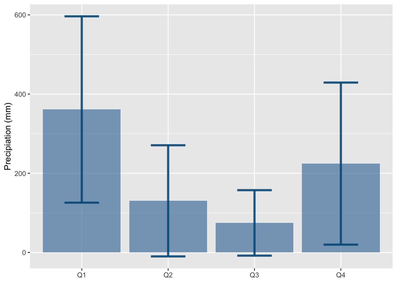
To convert the daily grid data into quarterly data, we aggregate the values on a quarter basis while preserving the spatial scale of the grid cells. Note: we only keep data from 1986 to 2015.
quarterly_weather_data <- weather_peru_daily_grid |>mutate(# year = lubridate::year(date),quarter = lubridate::quarter(date) ) |># Keeping 30 years of datafilter(year >=1986, year <=2015) |># Quartlery aggregates, at the grid cell levelgroup_by(year, quarter, grid_id) |>summarise(# Average min temperaturetemp_min =mean(temp_min, na.rm =TRUE),# Average max temperaturetemp_max =mean(temp_max, na.rm =TRUE),# Average mean temperaturetemp_mean =mean(temp_mean, na.rm =TRUE),# Total rainfallprecip_sum =sum(precip, na.rm =TRUE),# Total rainfall piscopprecip_piscop_sum =sum(precip_piscop, na.rm =TRUE),# Quarterly GDDgdd_rice =sum(gdd_daily_rice, na.rm =TRUE),gdd_maize =sum(gdd_daily_maize, na.rm =TRUE),gdd_potato =sum(gdd_daily_potato, na.rm =TRUE),gdd_cassava =sum(gdd_daily_cassava, na.rm =TRUE),# Quarterly HDDhdd_maize =sum(hdd_daily_maize, na.rm =TRUE),hdd_rice =sum(hdd_daily_rice, na.rm =TRUE),hdd_potato =sum(hdd_daily_potato, na.rm =TRUE),hdd_cassava =sum(hdd_daily_cassava, na.rm =TRUE) )
We do not need to keep track of the unit for the weather data. Let us drop that information.
To convert the daily grid data into annual data, we aggregate the values on an annual basis while preserving the spatial scale of the grid cells. Note: we only keep data from 1986 to 2015.
annual_weather_data <- weather_peru_daily_grid |>mutate(year = lubridate::year(date) ) |># Keeping 30 years of datafilter(year >=1986, year <=2015) |># Annual aggregates, at the grid cell levelgroup_by(year, grid_id) |>summarise(# Average min temperaturetemp_min =mean(temp_min, na.rm =TRUE),# Average max temperaturetemp_max =mean(temp_max, na.rm =TRUE),# Average mean temperaturetemp_mean =mean(temp_mean, na.rm =TRUE),# Total rainfallprecip_sum =sum(precip, na.rm =TRUE),# Total rainfall piscopprecip_piscop_sum =sum(precip_piscop, na.rm =TRUE),# Annual DDgdd_rice =sum(gdd_daily_rice, na.rm =TRUE),gdd_maize =sum(gdd_daily_maize, na.rm =TRUE),gdd_potato =sum(gdd_daily_potato, na.rm =TRUE),gdd_cassava =sum(gdd_daily_cassava, na.rm =TRUE),# Annual HDDhdd_maize =sum(hdd_daily_maize, na.rm =TRUE),hdd_rice =sum(hdd_daily_rice, na.rm =TRUE),hdd_potato =sum(hdd_daily_potato, na.rm =TRUE),hdd_cassava =sum(hdd_daily_cassava, na.rm =TRUE) )
We do not need to keep track of the unit for the weather data. Let us drop that information.
Burke, Gong, and Jones (2014) defines precipitation shocks as using a Gamma distribution. The historical data of monthly rainfall at each grid point are fitted to a grid-specific gamma distribution, and each year at the grid point is assigned to its corresponding percentile in that distribution. Note that Burke, Gong, and Jones (2014) uses crop-year data, whereas in our analysis, we use grid-month data.
We define a function, percentile_gamma_dist(), to estimate the parameters of a Gamma distribution using some input values. Then, for each input value, the corresponding percentile in the estimated distribution can be returned.
#' Estimate the shape and scale parameters of a Gamma distribution on the#' monthly sum of precipitation for a given cell, then returns the#' corresponding percentiles in the estimated distribution#' #' @param x data frame with `precip_sum`, for a cell in a given calendar monthpercentile_gamma_dist <-function(x, source =c("chirps", "piscop")) {# Estimate the shape and scale parameters of a Gamma distributionif (source =="chirps") { estim_gamma_precip <- EnvStats::egamma(x$precip_sum) } else { estim_gamma_precip <- EnvStats::egamma(x$precip_piscop_sum) } estim_g_shape <- estim_gamma_precip$parameters[["shape"]] estim_g_scale <- estim_gamma_precip$parameters[["scale"]]# Corresponding percentile in the estimated distributionpgamma(q = x$precip_sum, shape = estim_g_shape, scale = estim_g_scale)}
We aggregate the observations by grid cell and month. For each series of observations, we apply the percentile_gamma_dist() function.
To calculate evapotranspiration, we need to provide the latitude parameter to the thornthwaite() function from the {SPIE} package. For each grid cell, we use the latitude of its barycenter as the input.
We define a function, compute_spei_cell(), that computes the Potential evapotranspiration (PET), the Standardized Precipitation Index (SPI), and the Standardized Precipitation-Evapotranspiration Index (SPEI), at the grid level. We can specify, by giving a vector of integers to the scale argument, the time scale at which the SPI and the SPEI are computed. This scale argument controls for the magnitude of the memory. In the help file of {SPEI}, one can read:
The magnitude of this memory is controlled by parameter scale. For example, a value of six would imply that data from the current month and of the past five months will be used for computing the SPEI or SPI value for a given month.
#' Returns the SPI and SPEI on a monthly basis for a specific grid cell at#' different scales#'#' @param grid_id id of the grid cell#' @param scale vector of scales for the spi and spei functions#' @returns a tibble at the grid x monthly scale with the spi and the spei at#' different scalescompute_spei_cell <-function(grid_id, scale =c(1,3,6,12)) { lat <- centroids_grid |>filter(grid_id ==!!grid_id) |>pull(latitude) |>unique() |>as.numeric() tmp_grid <- monthly_weather_data |># Focus on grid cellfilter(grid_id ==!!grid_id) |>ungroup() |>arrange(year, month) |> dplyr::select( year, month, grid_id, precip_sum, precip_piscop_sum, temp_mean, latitude ) |>mutate(PET = SPEI::thornthwaite(temp_mean, lat, verbose =FALSE), BAL = precip_sum - PET,BAL_piscop = precip_piscop_sum - PET ) df_spi <-map(.x = scale,.f =~tibble(scale = .x,spi = SPEI::spi( tmp_grid$precip_sum, scale = .x, verbose =FALSE)$fitted,spei = SPEI::spei( tmp_grid$precip_sum, scale = .x, verbose =FALSE)$fitted,spi_piscop = SPEI::spi( tmp_grid$precip_piscop_sum, scale = .x, verbose =FALSE)$fitted,spei_piscop = SPEI::spei( tmp_grid$precip_piscop_sum, scale = .x, verbose =FALSE)$fitted ) |>mutate(t =row_number()) |>mutate(spi =ifelse(is.infinite(spi), yes =NA, no = spi),spei =ifelse(is.infinite(spei), yes =NA, no = spei),spi_piscop =ifelse(is.infinite(spi_piscop), yes =NA, no = spi_piscop),spei_piscop =ifelse(is.infinite(spei_piscop), yes =NA, no = spei_piscop) ) ) |>list_rbind() |>pivot_wider(names_from = scale, values_from =c(spi, spei, spi_piscop, spei_piscop)) |> dplyr::select(-t)bind_cols(tmp_grid, df_spi) |> dplyr::select(-precip_sum, -precip_piscop_sum, -temp_mean, -latitude)}
We can then apply the compute_spei_cell() function to all the grid cells
We now proceed to aggregate the monthly values of each grid cell to the scale of administrative regions. To accomplish this, for each region, we simply calculate the average of the values from each cell, weighting each term according to two measures. Firstly, the proportion that the cell represents in the total surface area of the region. Secondly, the proportion that the cell represents in the agricultural production of the region.
We define a function, aggregate_region_i(), to perform the aggregation for a specific region.
#' Aggregates the weather data at the region level#' @description For a specific region, the grid cells within that region are#' first identified. Then, the area of the intersection between each grid cell#' and the region are computed. The share of agricultural lands in each cell#' is also computed. Combined together, the area of the intersection and the#' agricultural share are used as weights to aggregate the data at the#' regional level.#'#' @param i row index of the region in `map_peru`#' @param weather_variables vector of name of the weather variables to aggregateaggregate_region_i <-function(i, weather_variables) { map_region_i <- map_peru[i,] tmp <- sf::st_intersection(map_peru_grid_agri, map_region_i) |># Get the area of the intersection between the polygon of the current# region and each grid cell that intersects it dplyr::mutate(area_cell_intersect = sf::st_area(geometry)) |> dplyr::rename(grid_id = i) |># Get the weather data for the corresponding grid cells dplyr::left_join( monthly_weather_data,by ="grid_id" ) |> dplyr::filter(!is.na(year)) |># Remove the unit in the area (squared metres) dplyr::mutate(area_cell_intersect = units::drop_units(area_cell_intersect) ) |> dplyr::group_by(month, year) |># Compute the weights to attribute to each grid cell dplyr::mutate(w_cropland = cropland /sum(cropland),w_area = area_cell_intersect /sum(area_cell_intersect),w = w_cropland * w_area,w = w /sum(w)) |># Weighted weather variables dplyr::mutate( dplyr::across(.cols =!!weather_variables,.fns =~ .x * w ) ) |> dplyr::select(-geometry) |> tibble::as_tibble() |> dplyr::group_by(year, month) |> dplyr::select(-geometry) |> tibble::as_tibble() |> dplyr::group_by(year, month) |> dplyr::summarise( dplyr::across(.cols =!!weather_variables,.fns =~sum(.x, na.rm =TRUE) ),.groups ="drop" ) |> dplyr::mutate(IDDPTO = map_region_i$IDDPTO)}
Then, we apply the aggregate_region_i() function to each region:
weather_regions_df <- weather_regions_df |> labelled::set_variable_labels(year ="Year",month ="Month",temp_min ="Min. Temperature",temp_max ="Max. Temperature",temp_mean ="Mean Temperature",precip_sum ="Total Rainfall (Chirps)",precip_piscop_sum ="Total Rainfall (Piscop)",perc_gamma_precip ="Precipitation Shock (Percentile from Gamma Dist., Chirps)",perc_gamma_precip_piscop ="Precipitation Shock (Percentile from Gamma Dist., Piscop)",temp_min_dev ="Deviation of Min. Temperature from Normals",temp_max_dev ="Deviation of Max. Temperature from Normals",temp_mean_dev ="Deviation of Mean Temperature from Normals",precip_sum_dev ="Deviation of Total Rainfall from Normals (Chirps)",precip_piscop_sum_dev ="Deviation of Total Rainfall from Normals (Piscop)",gdd_rice ="Degree Days",gdd_maize ="Degree Days",gdd_potato ="Degree Days",gdd_cassava ="Degree Days",hdd_rice ="Harmful Degree Days",hdd_maize ="Harmful Degree Days",hdd_potato ="Harmful Degree Days",hdd_cassava ="Harmful Degree Days",gdd_rice_dev ="Deviation of Degree Days from Normals",gdd_maize_dev ="Deviation of Degree Days from Normals",gdd_potato_dev ="Deviation of Degree Days from Normals",gdd_cassava_dev ="Deviation of Degree Days from Normals",hdd_rice_dev ="Deviation of Harmful Degree Days from Normals",hdd_maize_dev ="Deviation of Harmful Degree Days from Normals",hdd_potato_dev ="Deviation of Harmful Degree Days from Normals",hdd_cassava_dev ="Deviation of Harmful Degree Days from Normals",spi_1 ="SPI Index (scale = 1)",spi_3 ="SPI Index (scale = 3)",spi_6 ="SPI Index (scale = 6)",spi_12 ="SPI Index (scale = 12)",spei_1 ="SPEI Index (scale = 1)",spei_3 ="SPEI Index (scale = 3)",spei_6 ="SPEI Index (scale = 6)",spei_12 ="SPEI Index (scale = 12)",spi_piscop_1 ="SPI Index (scale = 1)",spi_piscop_3 ="SPI Index (scale = 3)",spi_piscop_6 ="SPI Index (scale = 6)",spi_piscop_12 ="SPI Index (scale = 12)",spei_piscop_1 ="SPEI Index (scale = 1)",spei_piscop_3 ="SPEI Index (scale = 3)",spei_piscop_6 ="SPEI Index (scale = 6)",spei_piscop_12 ="SPEI Index (scale = 12)",cold_surprise_maize ="Cold Surprise Weather", cold_surprise_rice ="Cold Surprise Weather", cold_surprise_potato ="Cold Surprise Weather", cold_surprise_cassava ="Cold Surprise Weather",hot_surprise_maize ="Hot Surprise Weather",hot_surprise_rice ="Hot Surprise Weather",hot_surprise_potato ="Hot Surprise Weather",hot_surprise_cassava ="Hot Surprise Weather",dry_surprise_maize ="Dry Surprise Weather", dry_surprise_rice ="Dry Surprise Weather", dry_surprise_potato ="Dry Surprise Weather", dry_surprise_cassava ="Dry Surprise Weather",wet_surprise_maize ="Wet Surprise Weather",wet_surprise_rice ="Wet Surprise Weather",wet_surprise_potato ="Wet Surprise Weather",wet_surprise_cassava ="Wet Surprise Weather",IDDPTO ="Region ID",DEPARTAMEN ="Region Name" )
We define a function, aggregate_quarter_region_i(), to perform the aggregation for a specific region.
#' Aggregates the weather data at the quarterly region level#' @description For a specific region, the grid cells within that region are#' first identified. Then, the area of the intersection between each grid cell#' and the region are computed. The share of agricultural lands in each cell#' is also computed. Combined together, the area of the intersection and the#' agricultural share are used as weights to aggregate the data at the#' regional level.#'#' @param i row index of the region in `map_peru`#' @param weather_variables vector of name of the weather variables to aggregateaggregate_quarter_region_i <-function(i, weather_variables) { map_region_i <- map_peru[i,] tmp <- sf::st_intersection(map_peru_grid_agri, map_region_i) |># Get the area of the intersection between the polygon of the current# region and each grid cell that intersects it dplyr::mutate(area_cell_intersect = sf::st_area(geometry)) |> dplyr::rename(grid_id = i) |># Get the weather data for the corresponding grid cells dplyr::left_join( quarterly_weather_data,by ="grid_id" ) |> dplyr::filter(!is.na(year)) |># Remove the unit in the area (squared metres) dplyr::mutate(area_cell_intersect = units::drop_units(area_cell_intersect) ) |> dplyr::group_by(quarter, year) |># Compute the weights to attribute to each grid cell dplyr::mutate(w_cropland = cropland /sum(cropland),w_area = area_cell_intersect /sum(area_cell_intersect),w = w_cropland * w_area,w = w /sum(w)) |># Weighted weather variables dplyr::mutate( dplyr::across(.cols =!!weather_variables,.fns =~ .x * w ) ) |> dplyr::select(-geometry) |> tibble::as_tibble() |> dplyr::group_by(year, quarter) |> dplyr::select(-geometry) |> tibble::as_tibble() |> dplyr::group_by(year, quarter) |> dplyr::summarise( dplyr::across(.cols =!!weather_variables,.fns =~sum(.x, na.rm =TRUE) ),.groups ="drop" ) |> dplyr::mutate(IDDPTO = map_region_i$IDDPTO)}
Then, we apply the aggregate_quarter_region_i() function to each region:
weather_quarter_regions_df <- weather_quarter_regions_df |> labelled::set_variable_labels(year ="Year",quarter ="Quarter",temp_min ="Min. Temperature",temp_max ="Max. Temperature",temp_mean ="Mean Temperature",precip_sum ="Total Rainfall (Chirps)",precip_piscop_sum ="Total Rainfall (Piscop)",perc_gamma_precip ="Precipitation Shock (Percentile from Gamma Dist., Chirps)",perc_gamma_precip_piscop ="Precipitation Shock (Percentile from Gamma Dist., Piscop)",temp_min_dev ="Deviation of Min. Temperature from Normals",temp_max_dev ="Deviation of Max. Temperature from Normals",temp_mean_dev ="Deviation of Mean Temperature from Normals",precip_sum_dev ="Deviation of Total Rainfall from Normals (Chirps)",precip_piscop_sum_dev ="Deviation of Total Rainfall from Normals (Piscop)",gdd_rice ="Degree Days",gdd_maize ="Degree Days",gdd_potato ="Degree Days",gdd_cassava ="Degree Days",hdd_rice ="Harmful Degree Days",hdd_maize ="Harmful Degree Days",hdd_potato ="Harmful Degree Days",hdd_cassava ="Harmful Degree Days",gdd_rice_dev ="Deviation of Degree Days from Normals",gdd_maize_dev ="Deviation of Degree Days from Normals",gdd_potato_dev ="Deviation of Degree Days from Normals",gdd_cassava_dev ="Deviation of Degree Days from Normals",hdd_rice_dev ="Deviation of Harmful Degree Days from Normals",hdd_maize_dev ="Deviation of Harmful Degree Days from Normals",hdd_potato_dev ="Deviation of Harmful Degree Days from Normals",hdd_cassava_dev ="Deviation of Harmful Degree Days from Normals",IDDPTO ="Region ID",DEPARTAMEN ="Region Name" )
We define a function, aggregate_annual_region_i(), to perform the aggregation for a specific region.
#' Aggregates the weather data at the annual region level#' @description For a specific region, the grid cells within that region are#' first identified. Then, the area of the intersection between each grid cell#' and the region are computed. The share of agricultural lands in each cell#' is also computed. Combined together, the area of the intersection and the#' agricultural share are used as weights to aggregate the data at the#' regional level.#'#' @param i row index of the region in `map_peru`#' @param weather_variables vector of name of the weather variables to aggregateaggregate_annual_region_i <-function(i, weather_variables) { map_region_i <- map_peru[i,] tmp <- sf::st_intersection(map_peru_grid_agri, map_region_i) |># Get the area of the intersection between the polygon of the current# region and each grid cell that intersects it dplyr::mutate(area_cell_intersect = sf::st_area(geometry)) |> dplyr::rename(grid_id = i) |># Get the weather data for the corresponding grid cells dplyr::left_join( annual_weather_data,by ="grid_id" ) |> dplyr::filter(!is.na(year)) |># Remove the unit in the area (squared metres) dplyr::mutate(area_cell_intersect = units::drop_units(area_cell_intersect) ) |> dplyr::group_by(year) |># Compute the weights to attribute to each grid cell dplyr::mutate(w_cropland = cropland /sum(cropland),w_area = area_cell_intersect /sum(area_cell_intersect),w = w_cropland * w_area,w = w /sum(w)) |># Weighted weather variables dplyr::mutate( dplyr::across(.cols =!!weather_variables,.fns =~ .x * w ) ) |> dplyr::select(-geometry) |> tibble::as_tibble() |> dplyr::group_by(year) |> dplyr::select(-geometry) |> tibble::as_tibble() |> dplyr::group_by(year) |> dplyr::summarise( dplyr::across(.cols =!!weather_variables,.fns =~sum(.x, na.rm =TRUE) ),.groups ="drop" ) |> dplyr::mutate(IDDPTO = map_region_i$IDDPTO)}
Then, we apply the aggregate_quarter_region_i() function to each region:
weather_annual_regions_df <- weather_annual_regions_df |> labelled::set_variable_labels(year ="Year",temp_min ="Min. Temperature",temp_max ="Max. Temperature",temp_mean ="Mean Temperature",precip_sum ="Total Rainfall (Chirps)",precip_piscop_sum ="Total Rainfall (Piscop)",perc_gamma_precip ="Precipitation Shock (Percentile from Gamma Dist., Chirps)",perc_gamma_precip_piscop ="Precipitation Shock (Percentile from Gamma Dist., Piscop)",temp_min_dev ="Deviation of Min. Temperature from Normals",temp_max_dev ="Deviation of Max. Temperature from Normals",temp_mean_dev ="Deviation of Mean Temperature from Normals",precip_sum_dev ="Deviation of Total Rainfall from Normals (Chirps)",precip_piscop_sum_dev ="Deviation of Total Rainfall from Normals (Piscop)",gdd_rice ="Growing Degree Days",gdd_maize ="Growing Degree Days",gdd_potato ="Growing Degree Days",gdd_cassava ="Growing Degree Days",hdd_rice ="Harmful Degree Days",hdd_maize ="Harmful Degree Days",hdd_potato ="Harmful Degree Days",hdd_cassava ="Harmful Degree Days",gdd_rice_dev ="Deviation of Growing Degree Days from Normals",gdd_maize_dev ="Deviation of Growing Degree Days from Normals",gdd_potato_dev ="Deviation of Growing Degree Days from Normals",gdd_cassava_dev ="Deviation of Growing Degree Days from Normals",hdd_rice_dev ="Deviation of Harmful Degree Days from Normals",hdd_maize_dev ="Deviation of Harmful Degree Days from Normals",hdd_potato_dev ="Deviation of Harmful Degree Days from Normals",hdd_cassava_dev ="Deviation of Harmful Degree Days from Normals",IDDPTO ="Region ID",DEPARTAMEN ="Region Name" )
Table 1.1: Variables in the weather_regions_df.rda file
Variable name
Type
Description
year
numeric
Year (YYYY)
month
numeric
Month (MM)
quarter
numeric
Quarter (1–4)
temp_min
numeric
Monthly average of daily min temperature
temp_max
numeric
Monthly average of daily max temperature
temp_mean
numeric
Monthly average of daily mean temperature
precip_sum
numeric
Monthly sum of daily rainfall
precip_piscop_sum
numeric
Monthly sum of daily rainfall (Piscop)
perc_gamma_precip
numeric
Percentile of the monthly precipitation (Estimated Gamma Distribution)
perc_gamma_precip_piscop
numeric
Percentile of the monthly precipitation (Estimated Gamma Distribution, Piscop)
temp_min_dev
numeric
Deviation of monthly min temperatures (temp_min) from climate normals (1986 – 2015)
temp_max_dev
numeric
Deviation of monthly max temperatures (temp_max) from climate normals (1986 – 2015)
temp_mean_dev
numeric
Deviation of monthly mean temperatures (temp_mean) from climate normals (1986 – 2015)
precip_sum_dev
numeric
Deviation of monthly total rainfall (precip_sum)
from climate normals (1986 – 2015)
precip_piscop_sum_dev
numeric
Deviation of monthly total rainfall (precip_sum, Piscop)
from climate normals (1986 – 2015)
spi_1, spi_piscop_1
numeric
SPI Drought Index, Scale = 1
spi_3, spi_piscop_3
numeric
SPI Drought Index, Scale = 3
spi_6, spi_piscop_6
numeric
SPI Drought Index, Scale = 6
spi_12, spi_piscop_12
numeric
SPI Drought Index, Scale = 12
spei_1, spei_piscop_1
numeric
SPEI Drought Index, Scale = 1
spei_3, spei_piscop_3
numeric
SPEI Drought Index, Scale = 3
spei_6, spei_piscop_6
numeric
SPEI Drought Index, Scale = 6
spei_12, spei_piscop_12
numeric
SPEI Drought Index, Scale = 12
IDDPTO
character
Region numerical ID
DEPARTAMEN
character
Region name
Aragón, Fernando M, Francisco Oteiza, and Juan Pablo Rud. 2021. “Climate Change and Agriculture: Subsistence Farmers’ Response to Extreme Heat.”American Economic Journal: Economic Policy 13 (1): 1–35. https://doi.org/10.1257/pol.20190316.
Aybar, Cesar, Carlos Fernández, Adrian Huerta, Waldo Lavado, Fiorella Vega, and Oscar Felipe-Obando. 2020. “Construction of a High-Resolution Gridded Rainfall Dataset for Peru from 1981 to the Present Day.”Hydrological Sciences Journal 65 (5): 770–85.
Burke, Marshall, Erick Gong, and Kelly Jones. 2014. “Income Shocks and HIV in Africa.”The Economic Journal 125 (585): 1157–89. https://doi.org/10.1111/ecoj.12149.
Funk, Chris, Pete Peterson, Martin Landsfeld, Diego Pedreros, James Verdin, Shraddhanand Shukla, Gregory Husak, et al. 2015. “CHIRPS: Rainfall Estimates from Rain Gauge and Satellite Observations.”https://doi.org/10.15780/G2RP4Q.