Table 6.2: Descriptive statistics for monthly production (in tons) per type of crop
Culture
Mean
Median
Standard Deviation
Min
Max
No. regions
No. obs.
Cassava
4,531.272
1,798.6500
7,109.64
0
57,135.0
20
3,600
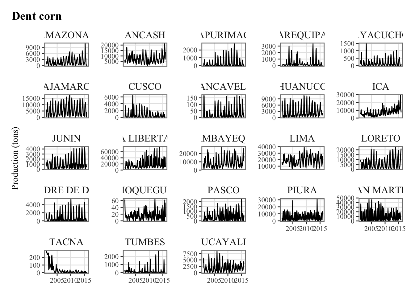
Dent corn
4,290.878
983.4735
7,254.97
0
74,623.7
23
4,140
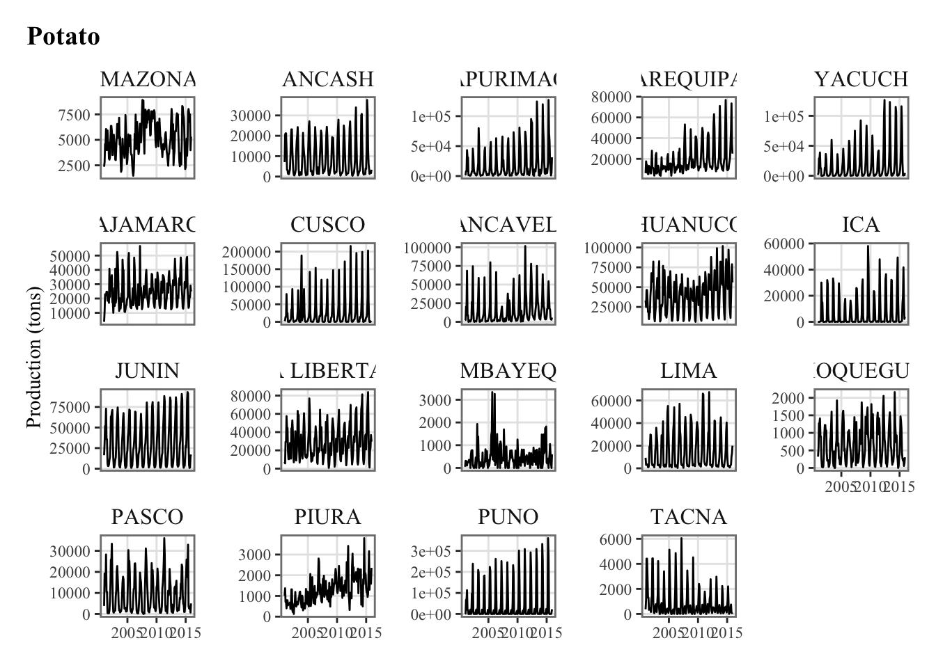
Potato
16,393.353
5,048.8500
29,574.83
0
360,070.0
19
3,420
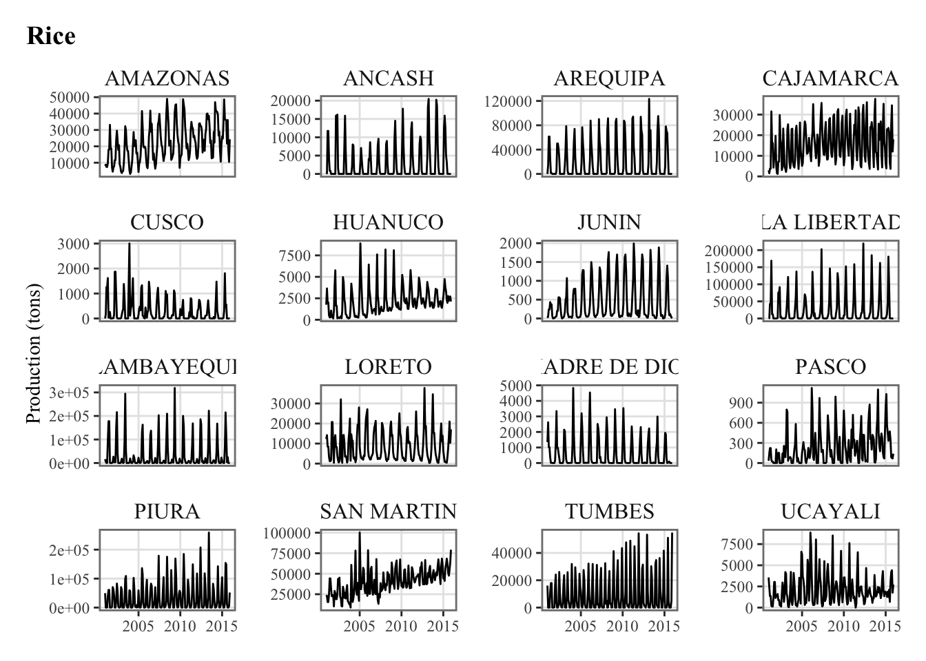
Rice
13,458.593
1,654.0000
28,312.71
0
318,706.0
16
2,880
6.2.1 National Production
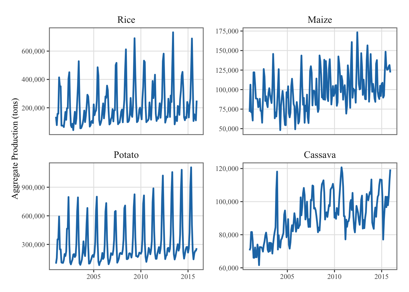
Figure 6.1 provides a visual representation of the national production of each time of crop over our time sample, which is the sum of the monthly regional production.
Figure 6.1: National monthly crop production for selected cultures (in tons)
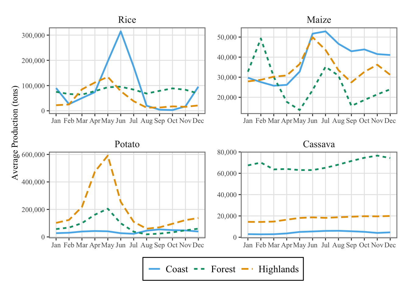
6.2.2 National Production by Month and Type of Region
In Figure 6.2, we document the regional differences and the seasonality by averaging the monthly production over the different types of natural regions.
Code
ggplot(data = df |>group_by(product_eng, year, month) |># Average each month at the national levelsummarise(prod_nat_costa =sum(y_new * share_costa),prod_nat_selva =sum(y_new * share_selva),prod_nat_sierra =sum(y_new * share_sierra),.groups ="drop" ) |>pivot_longer(cols =c(prod_nat_costa, prod_nat_selva, prod_nat_sierra),names_to ="geo",values_to ="monthly_prod_geo" ) |># Average in each region type for each calendar monthgroup_by(product_eng, month, geo) |>summarise(monthly_prod_geo =mean(monthly_prod_geo),.groups ="drop" ) |>mutate(product_eng =factor( product_eng, levels =c("Rice", "Dent corn", "Potato", "Cassava"),labels =c("Rice", "Maize", "Potato", "Cassava"), ),geo =factor( geo,levels =c("prod_nat_costa", "prod_nat_selva", "prod_nat_sierra"),labels =c("Coast", "Forest", "Highlands") ) ),mapping =aes(x = month, y = monthly_prod_geo, colour = geo, linetype = geo )) +geom_line(linewidth =1 ) +facet_wrap(~product_eng, scales ="free") +labs(x =NULL, y ="Average Production (tons)") +scale_colour_manual(NULL,values =c("Coast"="#56B4E9", "Forest"="#009E73", "Highlands"="#E69F00" ) ) +scale_linetype_discrete(NULL) +scale_x_continuous(breaks=1:12, labels = month.abb) +scale_y_continuous(labels = scales::number_format(big.mark =",")) +theme_paper()
Figure 6.2: Crop production by months and natural regions (in tons)
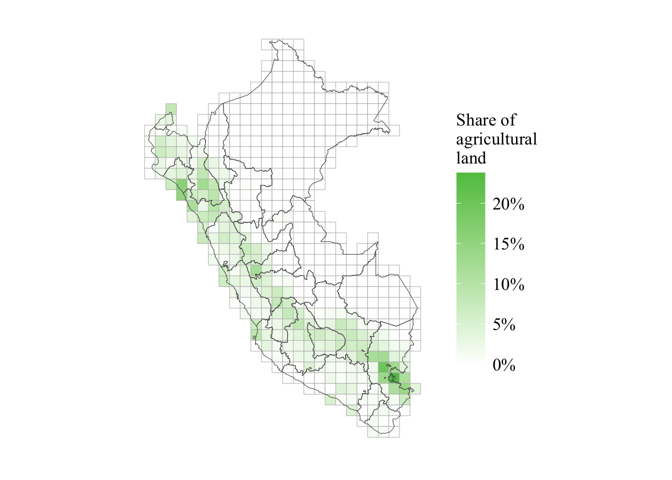
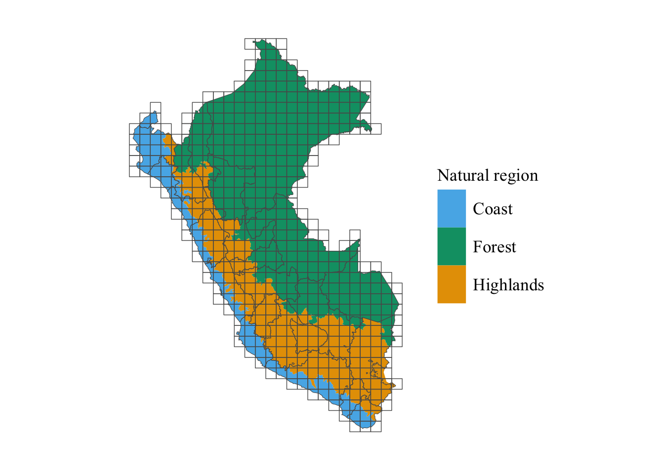
6.2.3 Share of agricultural land
Let us load the share of agricultural area in the cell, for each cell of the grid (see Section 1.2 for more details on that specific grid):
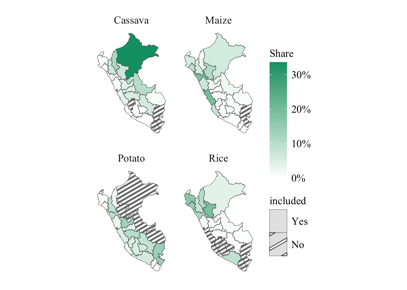
We can also look at the spatial distribution of these regions. Let us create a map that shows whether each region is included/excludes. On the same map, we would like to have an idea of the relative share in the total production over the period each region represents, for each crop.
Figure 6.5 shows these regions, and adds the grid used with the weather data from Chapter 1 as well as the regional boundaries used in the analysis.
Code
ggplot(data = map_regiones_naturales) +geom_sf(mapping =aes(fill = Natural_region), lwd =0) +scale_fill_manual(values = cols, name ="Natural region") +geom_sf(data = map_peru, fill =NA) +geom_sf(data = map_peru_grid_agri, fill =NA, lwd =0.25) +theme_map_paper()
Figure 6.5: Natural Regions in Peru
6.4 Correlations Between Agricultural Production and the Weather
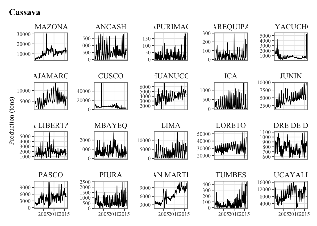
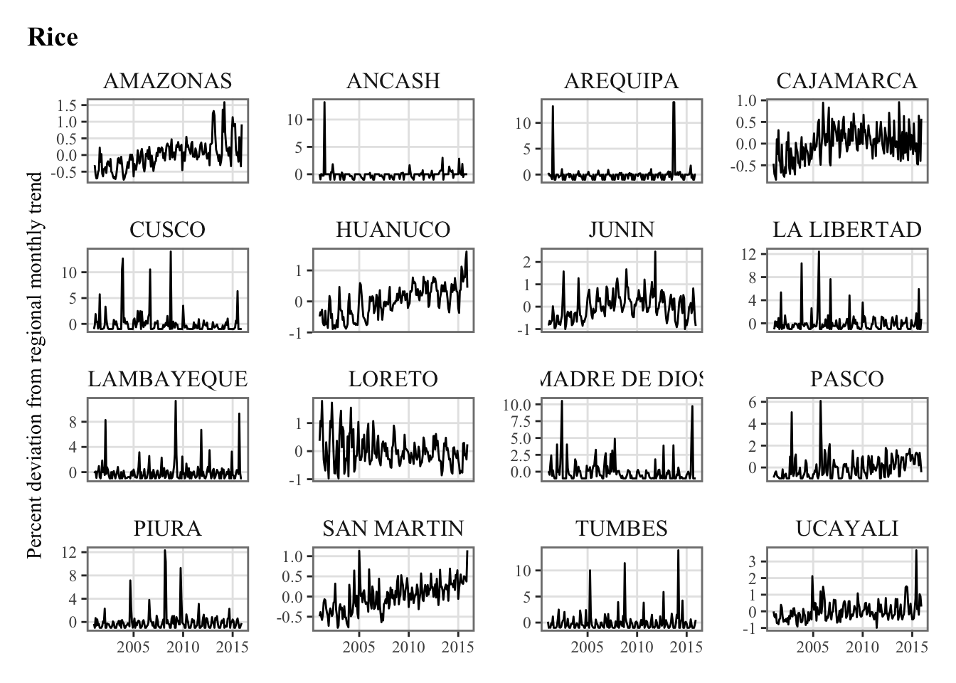
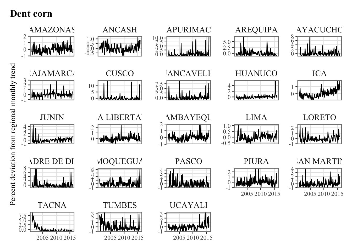
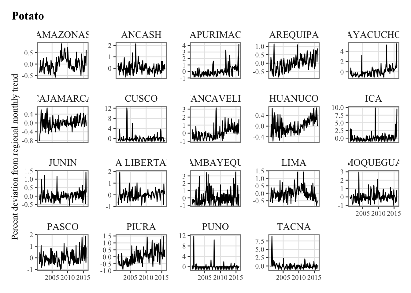
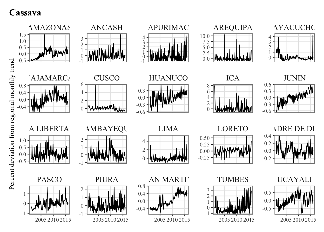
Let us compute the correlation between the agricultural production and our various weather variables. Recall from Chapter 5 that the agricultural production is defined as the percent deviation from the monthly trend.
plots_crops_lp <-vector(mode ="list", length =length(crops))for (i_crop in1:length(crops)) { current_crop <- crops[i_crop]# The series in each region for the current crop p_crop_lp <-ggplot(data = df |>filter(product_eng ==!!current_crop),mapping =aes(x = date, y = y_new) ) +geom_line() +facet_wrap(~region, scales ="free_y") +labs(title = current_crop, x =NULL,y ="Production (tons)") +theme_paper() plots_crops_lp[[i_crop]] <- p_crop_lp}names(plots_crops_lp) <- crops
plots_crops_lp <-vector(mode ="list", length =length(crops))for (i_crop in1:length(crops)) { current_crop <- crops[i_crop]# The series in each region for the current crop p_crop_lp <-ggplot(data = df |>filter(product_eng ==!!current_crop),mapping =aes(x = date, y = y_dev_pct) ) +geom_line() +facet_wrap(~region, scales ="free_y") +labs(title = current_crop, x =NULL,y ="Percent deviation from regional monthly trend") +theme_paper() plots_crops_lp[[i_crop]] <- p_crop_lp}names(plots_crops_lp) <- crops