10  From Regional to Aggregate Fluctuations

Objectives

This chapter investigates the transmission channels of a weather-induced shock in the agricultural production to the rest of the domestic economy.

library(tidyverse)
── Attaching core tidyverse packages ──────────────────────── tidyverse 2.0.0 ──
✔ dplyr     1.1.4     ✔ readr     2.1.5
✔ forcats   1.0.0     ✔ stringr   1.5.1
✔ ggplot2   3.5.1     ✔ tibble    3.2.1
✔ lubridate 1.9.3     ✔ tidyr     1.3.1
✔ purrr     1.0.2     
── Conflicts ────────────────────────────────────────── tidyverse_conflicts() ──
✖ dplyr::filter() masks stats::filter()
✖ dplyr::lag()    masks stats::lag()
ℹ Use the conflicted package (<http://conflicted.r-lib.org/>) to force all conflicts to become errors
library(labelled)

The {seasonal} and {timetk} packages are needed in this chapter, for seasonal adjustment by X-13 ARIMA-SEATS. If these packages are not installed:

# Do not run
install.packages("seasonal")
install.packages("timetk")

We will need the theme_paper() function to add our theme to the plots made with ggplot2. This function is defined in the utils.R script.

source("../weatherperu/R/utils.R")

10.1 Synthetic measure of the weather

This section provides a detailed description of the methodology employed to create the synthetic measure of the weather.

We need to load the results from the estimations made in Chapter 7.

load("../R/output/resul_lp_piscop.rda")
# Data used in the local projections
load("../data/output/df_lp.rda")

The average price of each crop in the data, denoted hereafter \(p_c\):

average_price_crops <- 
  df |> group_by(product_eng) |> 
  summarise(price_crop = mean(Value_prices, na.rm = TRUE))
average_price_crops
# A tibble: 4 × 2
  product_eng price_crop
  <chr>            <dbl>
1 Cassava          0.550
2 Dent corn        0.680
3 Potato           0.578
4 Rice             0.671

Then, we can put the coefficients in a table, for each crop and each time horizon:

weather_variables <- c(
  "temp_max_dev", "precip_piscop_sum_dev"
  )
coefs_weather <- map(
  .x = resul_lp,
  .f = ~ .x$coefs |> 
    filter(name %in% weather_variables) |> 
    select(horizon, name, value)
)
names(coefs_weather) <- map_chr(resul_lp, "crop_name")
coefs_weather <- 
  list_rbind(coefs_weather, names_to = "crop")

Then, we follow a methodology consisting of several key steps.

10.1.1 Step 1: Weather Shock Contribution

The first step involves estimating the contribution of weather shocks at each time period (\(t\)) for the chosen crop (\(c\)) and time horizon (\(h\)). This contribution is determined by considering the weather variables, temperature (\(T_{i,t}\)) and precipitation (\(P_{i,t}\)), and their respective coefficients (\(\beta_{c,h}^{T}\) as well as \(\beta_{c,h}^{P}\)). The weather shock contribution (\(\Gamma_{c,i,t,h}\)) is obtained by multiplying these coefficients with the corresponding weather variables and summing them up:

\[\Gamma_{c,i,t,h} = \beta_{c,h}^{T} T_{i,t-h} + \beta_{c,h}^{P} P_{i,t-h} \tag{10.1}\]

This first step is performed, using two user-defined functions: weather_contrib_crop_h() which computes the contribution of the weather for a single crop and time horizon, and with contrib_weather_crop() which uses the former to compute the contribution of the weather for a single crop, for all horizons considered. We will consider 9 horizons:

nb_periods_wcal <- 9
coefs_weather <- coefs_weather |>
  filter(horizon <= nb_periods_wcal)
#' Computes the contribution of the weather for a single crop and time horizon
#'
#' @param lp_crop LP for a specific crop
#' @param h horizon (single value)
#' @param weather_variables vector of names of the weather variables
#' @param ic_conf confidence interval used to determine whether a shock has a
#'   significant effect (default to .95)
weather_contrib_crop_h <- function(lp_crop,
                                   h,
                                   weather_variables,
                                   ic_conf = .95) {
  # The data
  data_lp <- lp_crop$data_lp
  data_lp <- data_lp[[which(names(data_lp) == h)]] |> 
    select(region_id, date, product_eng, !!weather_variables) |> 
    ungroup()
  # The coefficients
  lp_coefs <- 
    lp_crop$coefs |> 
    filter(horizon == !!h, name %in% !!weather_variables) |> 
    mutate(
      value_lb = value - qnorm(1 - ((1 - ic_conf) / 2)) * std,
      value_ub = value + qnorm(1 - ((1 - ic_conf) / 2)) * std
    )
  
  # Keeping the values
  lp_coefs_value <- lp_coefs$value
  # The lower and upper bounds
  lp_coefs_value_lb <- lp_coefs$value_lb
  lp_coefs_value_ub <- lp_coefs$value_ub
  
  data_lp |> 
    nest(.by = c(date, region_id)) |> 
    mutate(
      contribution = map(
        .x = data,
        .f = ~ as.matrix(.x[, weather_variables]) %*% lp_coefs_value |> 
          sum()
      ),
      contribution_lb = map(
        .x = data,
        .f = ~ as.matrix(.x[, weather_variables]) %*% lp_coefs_value_lb |> 
          sum()
      ),
      contribution_ub = map(
        .x = data,
        .f = ~ as.matrix(.x[, weather_variables]) %*% lp_coefs_value_ub |> 
          sum()
      )
    ) |> 
    unnest(cols = c(contribution, contribution_lb, contribution_ub)) |> 
    select(-data) |> 
    mutate(
      significant = (contribution_lb > 0 & contribution_ub > 0) | (contribution_lb < 0 & contribution_ub < 0),
      significant = as.numeric(significant)
    ) |> 
    mutate(date = date + lubridate::period(str_c(!!h, " month")))
}
#' Computes the contribution of the weather for a single crop, for all horizons
#'
#' @param lp_crop LP for a specific crop
#' @param weather_variables vector of names of the weather variables
#' @param horizons vector of horizons. If `NULL`, uses all horizons in lp_crop
contrib_weather_crop <- function(lp_crop,
                                 weather_variables,
                                 horizons = NULL) {
  if (is.null(horizons)) horizons <- unique(lp_crop$coefs$horizon)
  map(
    .x = horizons,
    .f = ~weather_contrib_crop_h(
      lp_crop = lp_crop, 
      h = .x, 
      weather_variables = weather_variables
    ) |> 
      mutate(horizon = .x)
  ) |> 
    list_rbind() |> 
    # group_by(date) |> 
    # summarise(value = sum(contribution)) |> 
    mutate(crop = lp_crop$crop_name) |> 
    mutate(contribution_signif = contribution * significant)
}

Let us compute the \(\Gamma_{c,i,t,h}\) for each crop, region, date and horizon:

weather_measure_crop <- 
  map(
    .x = resul_lp,
    .f = ~contrib_weather_crop(
      lp_crop = .x, 
      weather_variables = weather_variables,
      horizons = 0:nb_periods_wcal
    )
  ) |> 
  list_rbind()

Let us add the monthly regional selling prices of the crops (df$Value_prices), as well as the average crop-specific prices computed earlier on the whole sample (average_price_crops$price_crop) which will be used as a weight when we will aggregate all crops.

weather_measure_crop <- 
  weather_measure_crop |> 
  left_join(
    df |> select(product_eng, region_id, date, y_new, Value_prices),
    by = c("date", "crop" = "product_eng", "region_id")
  ) |> 
  left_join(
    average_price_crops,
    by = c("crop" = "product_eng")
  )

weather_measure_crop
# A tibble: 136,890 × 12
   date       region_id contribution contribution_lb contribution_ub significant
   <date>     <fct>            <dbl>           <dbl>           <dbl>       <dbl>
 1 2001-01-01 1              0.354           0.443            0.265            1
 2 2001-02-01 1              0.267           0.363            0.171            1
 3 2001-03-01 1              0.167           0.207            0.128            1
 4 2001-04-01 1              0.0955          0.138            0.0526           1
 5 2001-05-01 1              0.110           0.133            0.0874           1
 6 2001-06-01 1              0.197           0.256            0.138            1
 7 2001-07-01 1              0.116           0.147            0.0855           1
 8 2001-08-01 1              0.0466          0.0658           0.0275           1
 9 2001-09-01 1              0.124           0.136            0.113            1
10 2001-10-01 1              0.00941         0.00436          0.0145           1
# ℹ 136,880 more rows
# ℹ 6 more variables: horizon <int>, crop <chr>, contribution_signif <dbl>,
#   y_new <dbl>, Value_prices <dbl>, price_crop <dbl>

10.1.2 Step 2: Quantity Weights

For each crop and date \(t\), we define some weights for the regional observations using the data observed at horizon \(h=0\), as the sum of the monthly agricultural production over the regions considered in the analysis. The monthly production is expressed in monetary terms, by multiplying the quantities (y_new, i.e., \(y^{raw}\)) by unit price (price_crop, i.e., \(p_c\)).

\[\omega_{c,t} = \sum_{i} y^{\text{raw}}_{c,t,i} \times p_{c}\]

quantity_weight <- 
  weather_measure_crop |> 
  filter(horizon == 0) |> 
  group_by(crop, date, horizon, price_crop) |> 
  summarise(quantity_weight = sum(price_crop * y_new), .groups = "drop") |> 
  select(crop, date, quantity_weight)
quantity_weight
# A tibble: 720 × 3
   crop    date       quantity_weight
   <chr>   <date>               <dbl>
 1 Cassava 2001-01-01          38797.
 2 Cassava 2001-02-01          39625.
 3 Cassava 2001-03-01          44893.
 4 Cassava 2001-04-01          44893.
 5 Cassava 2001-05-01          41857.
 6 Cassava 2001-06-01          36333.
 7 Cassava 2001-07-01          36333.
 8 Cassava 2001-08-01          39766.
 9 Cassava 2001-09-01          36525.
10 Cassava 2001-10-01          36525.
# ℹ 710 more rows

10.1.3 Step 3: Crop-Specific Weather-Adjusted Agricultural Production

For each crop \(c\), at each date \(t\), we compute the weather-adjusted agricultural production, \(y_{c,t}^{\omega}\), as the sum of the significant crop-specific contributions of the weather to the agricultural production. The crop-specific contribution across regions is first aggregated at the national level, using an average of the crop and region-specific contribution of the weather to the monetary equivalence of the agricultural production.

\[y_{c,t}^{\omega} = \sum_{h}\sum_{i} \frac{\mathbb{1}_{\text{signif}_{c,i,t,h}} \times \gamma_{c,i,t,h} \times p_{c} \times y^{\text{raw}}_{c,t,i}}{\text{card}(I_{c,t})},\]

where \(\text{card(I)}\) is the number of regions that produce crop \(c\) at time \(t\). The characteristic function \(\mathbb{1}_{\text{signif}_{c,it,h}}\) is equal to 1 when the contribution is significantly different from 0 (using the 95% confidence intervals of the coefficients \(\beta_{c,h}^{T}\) and \(\beta_{c,h}^{P}\)), and is equal to 0 otherwise.

weather_adjusted_ag <- 
  weather_measure_crop |> 
  # each group: observations across regions, for a crop x date x horizon
  group_by(crop, date, horizon, price_crop) |> 
  # weather-adjusted agricultural production at each horizon
  # y_{c,t,h}^{w}
  summarise(
    y_w = sum(price_crop * contribution_signif *  y_new / n(), na.rm = TRUE),
    .groups = "drop"
  ) |> 
  group_by(crop, date) |> 
  # weather-adjusted agricultural production summed over horizons
  # y_{c,t}^{w}
  summarise(
    y_w = sum(y_w),
    .groups = "drop"
  )

10.1.4 Step 4: Aggregation at the National Level

Then, we aggregate the crop-specific weather-adjusted agricultural production at the national level using the following formula: \[y_{t}^{\omega} = \frac{\sum_{c} y_{c,t}^{\omega}}{\sum_{c}\omega_{c,t}},\]

where \(\omega_{c,t}\) are the quantity weights computed in the second step.

w_df <- 
  weather_adjusted_ag |> 
  left_join(quantity_weight, by = c("crop", "date")) |> 
  group_by(date) |> 
  summarise(
    w = sum(y_w) / sum(quantity_weight),
    .groups = "drop"
  )

10.1.5 Step 5: Detrending

Lastly, we express the national weather-adjusted production as a loss, and take it as a deviation from its trend:

\[ W_{t} = -100 \times (y_{t}^{\omega} - \overline{y_{t}^{\omega}}), \]

where \(y_{t}^{\omega}\) is the trend, obtained with the HP filter.

# Load detrending functions
source("../weatherperu/R/detrending.R")

w_df <- w_df |> 
  mutate(
    w_trend = hp_filter_trend(w, freq = 14400),
    w_dt = - 100 * (w - w_trend),
  )

10.2 Agricultural Production

In the second step in the creation of the synthetic measure of the weater, we computed quantity weights \(\omega_{c,t}\), which correspond to the agricultural production in month \(t\) for crop \(t\), expressed in monetary terms. Let us aggregate these values across crops to obtain a monthly agricultural production: \[y_t^{A} = \sum_{c}\omega_{c,t}.\]

We then express these as percentage deviation from their trend computed using the HP filter.

agricultural_output <- 
  quantity_weight |> 
  group_by(date) |> 
  summarise(quantity_weight = sum(quantity_weight), .groups = "drop") |> 
  mutate(
    # Remove seasonality
    q_sa = adj_season_X13(quantity_weight, ymd("2001-01-01")),
    # Extract trend
    q_sa_trend = hp_filter_trend(q_sa, freq = 14400),
    # Percentage dev. from trend
    q = 100 * log(q_sa / q_sa_trend)
  ) |> 
  select(date, q)

Note: this is actually not used.

10.3 Macroeconomic indicators

The vector of endogenous variables in the estimation, denoted as \(Y_t\), consists of eight variables: \(W_t\), \(RER_t\), \(\pi_t^{a}\), \(\pi_{t}\) , \(X_t\), \(y^A_t\), \(y_t\), and \(r_t\):

  • \(W_t\) represents the aggregate measure of weather-driven agricultural losses defined in Section 10.1, which quantifies the loss in agricultural value added due to weather shocks, expressed as a deviation from its trend. It is the focal variable of interest in this analysis.

  • \(RER_t\) denotes the Real Exchange Rate (RER), which reflects the relative value of the domestic currency against a basket of foreign currencies.

  • \(\pi^a_t\) corresponds to the percentage change of the Food Consumer Price Index (CPIA), which serves as a measure of food inflation.

  • \(\pi_t\) corresponds to the percentage change of the Consumer Price Index (CPI), which serves as a measure of inflation.

  • \(X_t\) denotes Exports.

  • \(y^A_t\) is the Agricultural production.

  • \(y_t\) represents the Gross Domestic Product (GDP), which serves as a measure of the overall economic activity and output in the country.

  • \(r_t\) is the nominal rate.

To construct the vectors \(Y_t\), we use data from the Central Reserve Bank of Perú.

The Real Exchange Rate (RER) data are obtained using the token PN01259PM, the Food Consumer Price Index (CPIA) data with token PN01336PM, the Consumer Price Index (CPI) data with token PN01270PM, the Exports data with token PN01461BM, the GDP data with token PN01773AM, the agricultural GDP with token PN01755AM, and the nominal rate with token PN07819NM.

Let us load the dataset of macroeconomic variables (see Chapter 3 for details on the construction of these variables).

load("../data/output/macro/df_macro.rda")

10.4 Merging the Data

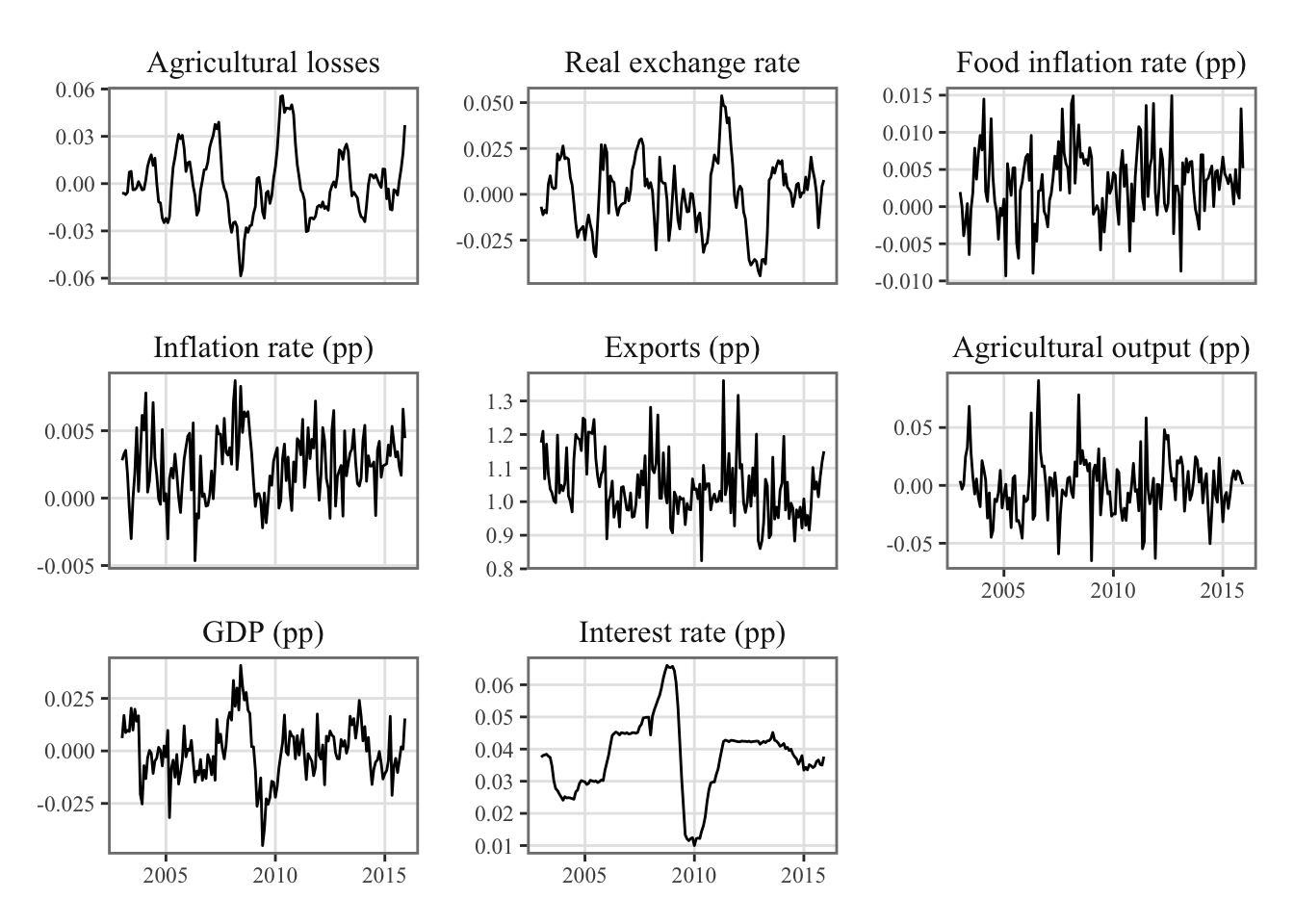
The sample period for our analysis covers the time span from January 2003 (2003M1) to December 2015 (2015M12). This period provides a comprehensive view of the relationship between weather-driven agricultural losses and the selected economic indicators in Peru.

df_var <- 
  df_macro |> 
  left_join(
    w_df,
    by = "date"
  ) |> 
  mutate(
    w = w_dt,
    q = ya
  )
  
variable_names <- c(
  "Agricultural losses" = "w",
  "Real exchange rate" = "rer_dt_sa",
  "Food inflation rate (pp)" = "pia",
  "Inflation rate (pp)" = "pi",
  "Exports (pp)" = "x",
  "Agricultural output (pp)" = "q",
  "GDP (pp)" = "y",
  "Interest rate (pp)" = "r"
)

Let us add labels to the new columns:

df_var <- 
  df_var |>  
  labelled::set_variable_labels(
    w = "Agricultural losses"
  )

Let us divide the all the values (except exports) by 100:

df_var <- 
  df_var |>  
  labelled::set_variable_labels(
    w = "Agricultural losses",
    q = "Agricultural output (pp)"
  ) |> 
  mutate(
    w = w / 100, 
    rer_dt_sa = rer_dt_sa / 100, 
    pi = pi / 100, 
    pia = pia / 100, 
    # x
    q = q / 100, 
    y = y / 100, 
    r = r / 100
  )

Figure Figure 17.1 displays the time series data for the variables included in the vector \(Y\).

ggplot(
    data = df_var |> 
      filter(date >= "2003-01-01") |> 
      select(date, w, rer_dt_sa, pia, pi, x, q, y, r) |> 
      pivot_longer(cols = -date) |> 
      mutate(
        name = factor(
          name,
          levels = variable_names,
          labels = names(variable_names)
        )
      ),
    mapping = aes(x = date, y = value)
  ) +
  geom_line() +
  facet_wrap(~name, scales = "free_y") +
  theme_paper() +
  labs(x = NULL, y = NULL)
Figure 10.1: Time Series of Endogenous Variables for Vector Autoregression (VAR) Analysis in Peru (2003-2015)

Before proceeding to the estimation, there is one final step, which involves converting the data into the ts format.

start_date <- "2003-01-01"
df_var_ts <-
  df_var |> 
  filter(date >= start_date) |> 
  select(
    w, rer_dt_sa, pia, pi, x, q, y, r
  ) |>
  ts(start = c(year(start_date), month(start_date)), freq = 12)

10.5 Estimation

We estimate a VAR(p) model with a constant term but no trend. Let us look how many lags we should use, using the automatic selection method provided by the VARselect() function from {vars}.

info_var_estim <- vars::VARselect(y = df_var_ts, type = "const", lag.max = 6)
info_var_estim
$selection
AIC(n)  HQ(n)  SC(n) FPE(n) 
     2      1      1      2 

$criteria
                   1             2             3             4             5
AIC(n) -7.720444e+01 -7.741493e+01 -7.702973e+01 -7.669223e+01 -7.650309e+01
HQ(n)  -7.661734e+01 -7.630596e+01 -7.539890e+01 -7.453952e+01 -7.382852e+01
SC(n)  -7.575933e+01 -7.468529e+01 -7.301555e+01 -7.139351e+01 -6.991984e+01
FPE(n)  2.958282e-34  2.412802e-34  3.608431e-34  5.228713e-34  6.678365e-34
                   6
AIC(n) -7.654810e+01
HQ(n)  -7.335167e+01
SC(n)  -6.868031e+01
FPE(n)  6.949015e-34

10.5.1 Results

Let us estimate a VAR(2) model with a constant term but no trend.

var_l1 <- vars::VAR(y = df_var_ts, p = 2, type = "const")
summary(var_l1)

VAR Estimation Results:
========================= 
Endogenous variables: w, rer_dt_sa, pia, pi, x, q, y, r 
Deterministic variables: const 
Sample size: 154 
Log Likelihood: 4342.644 
Roots of the characteristic polynomial:
0.8901 0.8901 0.8293 0.8293 0.5375 0.5375 0.4283 0.4013 0.4013 0.377 0.377 0.2778 0.2762 0.2762 0.2703 0.2703
Call:
vars::VAR(y = df_var_ts, p = 2, type = "const")


Estimation results for equation w: 
================================== 
w = w.l1 + rer_dt_sa.l1 + pia.l1 + pi.l1 + x.l1 + q.l1 + y.l1 + r.l1 + w.l2 + rer_dt_sa.l2 + pia.l2 + pi.l2 + x.l2 + q.l2 + y.l2 + r.l2 + const 

              Estimate Std. Error t value Pr(>|t|)    
w.l1          1.267638   0.078368  16.175  < 2e-16 ***
rer_dt_sa.l1  0.068611   0.062152   1.104   0.2716    
pia.l1       -0.059921   0.254887  -0.235   0.8145    
pi.l1         0.365242   0.529096   0.690   0.4912    
x.l1         -0.006021   0.007015  -0.858   0.3923    
q.l1          0.034348   0.026556   1.293   0.1980    
y.l1         -0.151286   0.062832  -2.408   0.0174 *  
r.l1          0.495312   0.313629   1.579   0.1166    
w.l2         -0.448714   0.079797  -5.623 1.01e-07 ***
rer_dt_sa.l2 -0.143152   0.064470  -2.220   0.0280 *  
pia.l2       -0.328037   0.253830  -1.292   0.1984    
pi.l2         0.374000   0.521350   0.717   0.4744    
x.l2         -0.006520   0.006740  -0.967   0.3351    
q.l2         -0.037625   0.026388  -1.426   0.1562    
y.l2          0.012412   0.064949   0.191   0.8487    
r.l2         -0.607335   0.306618  -1.981   0.0496 *  
const         0.016888   0.009983   1.692   0.0930 .  
---
Signif. codes:  0 '***' 0.001 '**' 0.01 '*' 0.05 '.' 0.1 ' ' 1


Residual standard error: 0.007158 on 137 degrees of freedom
Multiple R-Squared: 0.9002, Adjusted R-squared: 0.8886 
F-statistic: 77.25 on 16 and 137 DF,  p-value: < 2.2e-16 


Estimation results for equation rer_dt_sa: 
========================================== 
rer_dt_sa = w.l1 + rer_dt_sa.l1 + pia.l1 + pi.l1 + x.l1 + q.l1 + y.l1 + r.l1 + w.l2 + rer_dt_sa.l2 + pia.l2 + pi.l2 + x.l2 + q.l2 + y.l2 + r.l2 + const 

              Estimate Std. Error t value Pr(>|t|)    
w.l1         -0.128434   0.104940  -1.224   0.2231    
rer_dt_sa.l1  1.014179   0.083226  12.186   <2e-16 ***
pia.l1        0.429770   0.341311   1.259   0.2101    
pi.l1        -0.950152   0.708494  -1.341   0.1821    
x.l1          0.013879   0.009394   1.478   0.1418    
q.l1         -0.016263   0.035560  -0.457   0.6482    
y.l1          0.092633   0.084136   1.101   0.2728    
r.l1         -0.383389   0.419970  -0.913   0.3629    
w.l2          0.219431   0.106853   2.054   0.0419 *  
rer_dt_sa.l2 -0.188915   0.086329  -2.188   0.0303 *  
pia.l2        0.043780   0.339895   0.129   0.8977    
pi.l2         0.213844   0.698122   0.306   0.7598    
x.l2         -0.014129   0.009025  -1.566   0.1198    
q.l2         -0.003499   0.035336  -0.099   0.9213    
y.l2         -0.005852   0.086971  -0.067   0.9465    
r.l2          0.429207   0.410582   1.045   0.2977    
const        -0.001024   0.013368  -0.077   0.9391    
---
Signif. codes:  0 '***' 0.001 '**' 0.01 '*' 0.05 '.' 0.1 ' ' 1


Residual standard error: 0.009585 on 137 degrees of freedom
Multiple R-Squared: 0.782,  Adjusted R-squared: 0.7565 
F-statistic: 30.71 on 16 and 137 DF,  p-value: < 2.2e-16 


Estimation results for equation pia: 
==================================== 
pia = w.l1 + rer_dt_sa.l1 + pia.l1 + pi.l1 + x.l1 + q.l1 + y.l1 + r.l1 + w.l2 + rer_dt_sa.l2 + pia.l2 + pi.l2 + x.l2 + q.l2 + y.l2 + r.l2 + const 

               Estimate Std. Error t value Pr(>|t|)  
w.l1          0.0052509  0.0493833   0.106   0.9155  
rer_dt_sa.l1  0.0580618  0.0391649   1.482   0.1405  
pia.l1        0.1803229  0.1606159   1.123   0.2635  
pi.l1         0.0866057  0.3334069   0.260   0.7954  
x.l1         -0.0051089  0.0044205  -1.156   0.2498  
q.l1         -0.0184108  0.0167340  -1.100   0.2732  
y.l1          0.0069203  0.0395932   0.175   0.8615  
r.l1         -0.0621598  0.1976318  -0.315   0.7536  
w.l2         -0.0188948  0.0502835  -0.376   0.7077  
rer_dt_sa.l2 -0.0074583  0.0406251  -0.184   0.8546  
pia.l2       -0.0159533  0.1599494  -0.100   0.9207  
pi.l2         0.0492539  0.3285258   0.150   0.8810  
x.l2          0.0024291  0.0042471   0.572   0.5683  
q.l2          0.0004987  0.0166285   0.030   0.9761  
y.l2          0.0821621  0.0409271   2.008   0.0467 *
r.l2          0.0274411  0.1932138   0.142   0.8873  
const         0.0065104  0.0062906   1.035   0.3025  
---
Signif. codes:  0 '***' 0.001 '**' 0.01 '*' 0.05 '.' 0.1 ' ' 1


Residual standard error: 0.00451 on 137 degrees of freedom
Multiple R-Squared: 0.1951, Adjusted R-squared: 0.1011 
F-statistic: 2.075 on 16 and 137 DF,  p-value: 0.01265 


Estimation results for equation pi: 
=================================== 
pi = w.l1 + rer_dt_sa.l1 + pia.l1 + pi.l1 + x.l1 + q.l1 + y.l1 + r.l1 + w.l2 + rer_dt_sa.l2 + pia.l2 + pi.l2 + x.l2 + q.l2 + y.l2 + r.l2 + const 

               Estimate Std. Error t value Pr(>|t|)  
w.l1          0.0097926  0.0239830   0.408    0.684  
rer_dt_sa.l1  0.0455393  0.0190204   2.394    0.018 *
pia.l1       -0.0273362  0.0780032  -0.350    0.727  
pi.l1         0.2660423  0.1619191   1.643    0.103  
x.l1         -0.0018619  0.0021468  -0.867    0.387  
q.l1         -0.0122134  0.0081268  -1.503    0.135  
y.l1          0.0265333  0.0192284   1.380    0.170  
r.l1         -0.0001969  0.0959799  -0.002    0.998  
w.l2         -0.0217587  0.0244202  -0.891    0.374  
rer_dt_sa.l2 -0.0161181  0.0197296  -0.817    0.415  
pia.l2        0.0124399  0.0776795   0.160    0.873  
pi.l2        -0.0370116  0.1595486  -0.232    0.817  
x.l2          0.0009803  0.0020626   0.475    0.635  
q.l2         -0.0007480  0.0080756  -0.093    0.926  
y.l2          0.0362947  0.0198762   1.826    0.070 .
r.l2         -0.0213335  0.0938343  -0.227    0.820  
const         0.0036878  0.0030550   1.207    0.229  
---
Signif. codes:  0 '***' 0.001 '**' 0.01 '*' 0.05 '.' 0.1 ' ' 1


Residual standard error: 0.002191 on 137 degrees of freedom
Multiple R-Squared:  0.28,  Adjusted R-squared: 0.1959 
F-statistic:  3.33 on 16 and 137 DF,  p-value: 6.3e-05 


Estimation results for equation x: 
================================== 
x = w.l1 + rer_dt_sa.l1 + pia.l1 + pi.l1 + x.l1 + q.l1 + y.l1 + r.l1 + w.l2 + rer_dt_sa.l2 + pia.l2 + pi.l2 + x.l2 + q.l2 + y.l2 + r.l2 + const 

             Estimate Std. Error t value Pr(>|t|)    
w.l1         -0.72984    0.96318  -0.758   0.4499    
rer_dt_sa.l1 -0.29342    0.76388  -0.384   0.7015    
pia.l1       -1.33995    3.13267  -0.428   0.6695    
pi.l1         5.28399    6.50280   0.813   0.4179    
x.l1          0.14367    0.08622   1.666   0.0979 .  
q.l1         -0.46358    0.32638  -1.420   0.1578    
y.l1          1.06544    0.77223   1.380   0.1699    
r.l1         -0.59428    3.85463  -0.154   0.8777    
w.l2         -0.28340    0.98073  -0.289   0.7730    
rer_dt_sa.l2  0.13202    0.79236   0.167   0.8679    
pia.l2       -1.66568    3.11967  -0.534   0.5943    
pi.l2         4.34184    6.40760   0.678   0.4992    
x.l2          0.14425    0.08284   1.741   0.0839 .  
q.l2         -0.10515    0.32432  -0.324   0.7463    
y.l2          0.24162    0.79825   0.303   0.7626    
r.l2         -1.29717    3.76846  -0.344   0.7312    
const         0.79948    0.12269   6.516 1.27e-09 ***
---
Signif. codes:  0 '***' 0.001 '**' 0.01 '*' 0.05 '.' 0.1 ' ' 1


Residual standard error: 0.08797 on 137 degrees of freedom
Multiple R-Squared: 0.2248, Adjusted R-squared: 0.1343 
F-statistic: 2.484 on 16 and 137 DF,  p-value: 0.002373 


Estimation results for equation q: 
================================== 
q = w.l1 + rer_dt_sa.l1 + pia.l1 + pi.l1 + x.l1 + q.l1 + y.l1 + r.l1 + w.l2 + rer_dt_sa.l2 + pia.l2 + pi.l2 + x.l2 + q.l2 + y.l2 + r.l2 + const 

              Estimate Std. Error t value Pr(>|t|)  
w.l1         -0.362386   0.259425  -1.397    0.165  
rer_dt_sa.l1 -0.178436   0.205745  -0.867    0.387  
pia.l1       -0.407730   0.843764  -0.483    0.630  
pi.l1        -0.986757   1.751487  -0.563    0.574  
x.l1         -0.004487   0.023222  -0.193    0.847  
q.l1          0.197841   0.087909   2.251    0.026 *
y.l1          0.095053   0.207995   0.457    0.648  
r.l1          0.790868   1.038220   0.762    0.448  
w.l2          0.060895   0.264154   0.231    0.818  
rer_dt_sa.l2  0.015055   0.213416   0.071    0.944  
pia.l2       -1.164964   0.840263  -1.386    0.168  
pi.l2         1.311820   1.725846   0.760    0.448  
x.l2         -0.023495   0.022312  -1.053    0.294  
q.l2         -0.127431   0.087354  -1.459    0.147  
y.l2         -0.044173   0.215002  -0.205    0.838  
r.l2         -0.436027   1.015011  -0.430    0.668  
const         0.019718   0.033046   0.597    0.552  
---
Signif. codes:  0 '***' 0.001 '**' 0.01 '*' 0.05 '.' 0.1 ' ' 1


Residual standard error: 0.0237 on 137 degrees of freedom
Multiple R-Squared: 0.2203, Adjusted R-squared: 0.1292 
F-statistic: 2.419 on 16 and 137 DF,  p-value: 0.00311 


Estimation results for equation y: 
================================== 
y = w.l1 + rer_dt_sa.l1 + pia.l1 + pi.l1 + x.l1 + q.l1 + y.l1 + r.l1 + w.l2 + rer_dt_sa.l2 + pia.l2 + pi.l2 + x.l2 + q.l2 + y.l2 + r.l2 + const 

              Estimate Std. Error t value Pr(>|t|)    
w.l1         -0.003199   0.109057  -0.029  0.97664    
rer_dt_sa.l1 -0.038732   0.086491  -0.448  0.65499    
pia.l1        0.211133   0.354701   0.595  0.55266    
pi.l1         0.598298   0.736289   0.813  0.41787    
x.l1         -0.004104   0.009762  -0.420  0.67487    
q.l1          0.034623   0.036955   0.937  0.35047    
y.l1          0.415904   0.087437   4.757 4.93e-06 ***
r.l1          0.324613   0.436446   0.744  0.45829    
w.l2          0.051638   0.111045   0.465  0.64265    
rer_dt_sa.l2  0.003376   0.089716   0.038  0.97004    
pia.l2       -0.210002   0.353229  -0.595  0.55315    
pi.l2         0.202028   0.725510   0.278  0.78108    
x.l2          0.012840   0.009379   1.369  0.17324    
q.l2          0.010711   0.036722   0.292  0.77096    
y.l2          0.250580   0.090383   2.772  0.00634 ** 
r.l2         -0.302527   0.426689  -0.709  0.47952    
const        -0.012004   0.013892  -0.864  0.38907    
---
Signif. codes:  0 '***' 0.001 '**' 0.01 '*' 0.05 '.' 0.1 ' ' 1


Residual standard error: 0.009961 on 137 degrees of freedom
Multiple R-Squared: 0.5263, Adjusted R-squared: 0.471 
F-statistic: 9.513 on 16 and 137 DF,  p-value: 1.514e-15 


Estimation results for equation r: 
================================== 
r = w.l1 + rer_dt_sa.l1 + pia.l1 + pi.l1 + x.l1 + q.l1 + y.l1 + r.l1 + w.l2 + rer_dt_sa.l2 + pia.l2 + pi.l2 + x.l2 + q.l2 + y.l2 + r.l2 + const 

               Estimate Std. Error t value Pr(>|t|)    
w.l1          6.421e-03  1.833e-02   0.350   0.7266    
rer_dt_sa.l1  8.568e-03  1.454e-02   0.589   0.5565    
pia.l1        1.247e-03  5.961e-02   0.021   0.9833    
pi.l1         3.173e-02  1.237e-01   0.256   0.7980    
x.l1         -1.024e-05  1.641e-03  -0.006   0.9950    
q.l1          2.224e-03  6.211e-03   0.358   0.7209    
y.l1          1.710e-02  1.469e-02   1.164   0.2466    
r.l1          1.452e+00  7.335e-02  19.795  < 2e-16 ***
w.l2         -4.633e-04  1.866e-02  -0.025   0.9802    
rer_dt_sa.l2 -8.438e-03  1.508e-02  -0.560   0.5767    
pia.l2       -7.185e-03  5.936e-02  -0.121   0.9038    
pi.l2         1.998e-01  1.219e-01   1.639   0.1035    
x.l2          5.996e-04  1.576e-03   0.380   0.7042    
q.l2         -4.738e-03  6.172e-03  -0.768   0.4440    
y.l2          2.734e-02  1.519e-02   1.800   0.0741 .  
r.l2         -5.101e-01  7.171e-02  -7.114 5.72e-11 ***
const         1.049e-03  2.335e-03   0.449   0.6540    
---
Signif. codes:  0 '***' 0.001 '**' 0.01 '*' 0.05 '.' 0.1 ' ' 1


Residual standard error: 0.001674 on 137 degrees of freedom
Multiple R-Squared: 0.9819, Adjusted R-squared: 0.9798 
F-statistic: 463.8 on 16 and 137 DF,  p-value: < 2.2e-16 


Covariance matrix of residuals:
                   w  rer_dt_sa        pia         pi          x          q
w          5.124e-05 -6.385e-06  1.420e-06 -1.763e-07  2.399e-05  1.197e-05
rer_dt_sa -6.385e-06  9.187e-05 -3.941e-06 -2.456e-06 -3.212e-05  1.313e-05
pia        1.420e-06 -3.941e-06  2.034e-05  8.375e-06 -2.967e-05  3.334e-06
pi        -1.763e-07 -2.456e-06  8.375e-06  4.798e-06 -2.648e-05  3.513e-06
x          2.399e-05 -3.212e-05 -2.967e-05 -2.648e-05  7.739e-03 -3.289e-04
q          1.197e-05  1.313e-05  3.334e-06  3.513e-06 -3.289e-04  5.615e-04
y         -1.998e-06  6.141e-06  1.200e-06  1.972e-06 -5.098e-05  6.238e-05
r          4.063e-07  5.816e-07  1.953e-06  8.293e-07 -9.949e-06  1.473e-06
                   y          r
w         -1.998e-06  4.063e-07
rer_dt_sa  6.141e-06  5.816e-07
pia        1.200e-06  1.953e-06
pi         1.972e-06  8.293e-07
x         -5.098e-05 -9.949e-06
q          6.238e-05  1.473e-06
y          9.922e-05  3.801e-06
r          3.801e-06  2.802e-06

Correlation matrix of residuals:
                 w rer_dt_sa      pia       pi        x        q        y
w          1.00000  -0.09307  0.04399 -0.01124  0.03809  0.07060 -0.02802
rer_dt_sa -0.09307   1.00000 -0.09116 -0.11698 -0.03809  0.05781  0.06432
pia        0.04399  -0.09116  1.00000  0.84767 -0.07477  0.03119  0.02671
pi        -0.01124  -0.11698  0.84767  1.00000 -0.13741  0.06768  0.09036
x          0.03809  -0.03809 -0.07477 -0.13741  1.00000 -0.15780 -0.05818
q          0.07060   0.05781  0.03119  0.06768 -0.15780  1.00000  0.26430
y         -0.02802   0.06432  0.02671  0.09036 -0.05818  0.26430  1.00000
r          0.03391   0.03625  0.25864  0.22616 -0.06755  0.03713  0.22796
                 r
w          0.03391
rer_dt_sa  0.03625
pia        0.25864
pi         0.22616
x         -0.06755
q          0.03713
y          0.22796
r          1.00000

10.5.2 Restricted VAR

We impose some restrictions on the VAR:

a <- diag(1, 8)
a[lower.tri(a)] <- NA
a
     [,1] [,2] [,3] [,4] [,5] [,6] [,7] [,8]
[1,]    1    0    0    0    0    0    0    0
[2,]   NA    1    0    0    0    0    0    0
[3,]   NA   NA    1    0    0    0    0    0
[4,]   NA   NA   NA    1    0    0    0    0
[5,]   NA   NA   NA   NA    1    0    0    0
[6,]   NA   NA   NA   NA   NA    1    0    0
[7,]   NA   NA   NA   NA   NA   NA    1    0
[8,]   NA   NA   NA   NA   NA   NA   NA    1
svar_a <- vars::SVAR(var_l1, Amat = a, max.iter = 500)
Warning in vars::SVAR(var_l1, Amat = a, max.iter = 500): Convergence not
achieved after 500 iterations. Convergence value: 8.95155527022712e-05 .

The matrix of the estimated coefficients:

svar_a$A
                   w  rer_dt_sa        pia         pi           x          q
w         1.00000000 0.00000000 0.00000000 0.00000000 0.000000000 0.00000000
rer_dt_sa 0.10062174 1.00000000 0.00000000 0.00000000 0.000000000 0.00000000
pia       0.09683520 0.09746244 1.00000000 0.00000000 0.000000000 0.00000000
pi        0.09696978 0.09646253 0.09446819 1.00000000 0.000000000 0.00000000
x         0.08956979 0.11302010 0.11451975 0.11371938 1.000000000 0.00000000
q         0.08405673 0.08343476 0.09004483 0.09074844 0.043870980 1.00000000
y         0.08370154 0.07915368 0.08356944 0.08389639 0.010703005 0.04580249
r         0.08307618 0.08163940 0.08355461 0.08470402 0.007045767 0.06823200
                  y r
w         0.0000000 0
rer_dt_sa 0.0000000 0
pia       0.0000000 0
pi        0.0000000 0
x         0.0000000 0
q         0.0000000 0
y         1.0000000 0
r         0.0839859 1
save(svar_a, df_var, file = "../R/output/var_objects_piscop.rda")

10.5.3 Impulse Response Functions

Let us focus on the impulse to the weather aggregate cost equation, with 95% confidence bootstrapped error bands (500 runs).

impulse_name <- "w"
nb_runs <- 500

irfs_95 <- vars::irf(
  svar_a, impulse = impulse_name, boot = TRUE, ci = .95, 
  n.ahead = 20, runs = nb_runs
)

And with 68% confidence bootstrapped error bands (500 runs, again).

irfs_68 <- vars::irf(
  svar_a, impulse = impulse_name, boot = TRUE, ci = .68, 
  n.ahead = 20, runs = nb_runs
)

Let us save the results:

save(irfs_95, file = "../R/output/irfs_95_piscop.rda")
save(irfs_68, file = "../R/output/irfs_68_piscop.rda")
levels <- variable_names
labels <- names(variable_names)

Now, we can plot the resulting IRFs. Let us prepare the data for the response:

df_irfs <- 
  irfs_95$irf[[impulse_name]] |> 
  as_tibble() |> 
  mutate(horizon = row_number()) |> 
  pivot_longer(cols = -horizon) |> 
  mutate(impulse = !!impulse_name)

df_irfs <- 
  df_irfs |> 
  mutate(
    name = factor(
      name,
      levels = !!levels,
      labels = !!labels
    )
  )

The error bands:

df_irfs_ci <- 
  map(
    .x = list(`95` = irfs_95, `68` = irfs_68),
    .f = function(irf_lvl) {
      map(
        .x = list(
          lower = irf_lvl$Lower[[impulse_name]], 
          mean = irf_lvl$irf[[impulse_name]],
          upper = irf_lvl$Upper[[impulse_name]]),
        .f = ~ .x |> 
          as_tibble() |> 
          mutate(horizon = row_number()) |> 
          pivot_longer(cols = -horizon, values_to = "bound") |> 
          mutate(impulse = !!impulse_name)
      ) |> 
        list_rbind(names_to = "bound_type")
    }
  ) |> 
  list_rbind(names_to = "level") |> 
  pivot_wider(names_from = bound_type, values_from = bound)

df_irfs_ci <- 
  df_irfs_ci |> 
  mutate(
    name = factor(
      name,
      levels = !!levels,
      labels = !!labels),
    level = factor(level, levels = c(68, 95), labels = c("68%", "95%"))
  )

And lastly, the graph.

ggplot() +
  geom_ribbon(
    data = df_irfs_ci,
    mapping = aes(
      x = horizon,
      ymin = lower, ymax = upper,
      fill = level),
    alpha = .3
  ) +
  geom_line(
    data = df_irfs_ci,
    mapping = aes(x = horizon, y = mean),
    colour = "#0072B2"
  ) +
  geom_hline(yintercept = 0, colour = "#444444") +
  labs(x = "Horizon", y = NULL) +
  scale_fill_manual(
    "C.I. level", 
    values = c("68%" = "#0072B2", "95%" = "#56B4E9")) +
  facet_wrap(~name, scales = "free_y", ncol = 4) +
  theme_paper() +
  coord_cartesian(xlim = c(1, 20))
Figure 10.2: VAR(2) system response to one standard deviation orthogonal shock to the weather aggregate cost equation

The exact figure replication:

Code
library(tikzDevice)
library(lemon)

ggplot() +
  geom_ribbon(
    data = df_irfs_ci |> 
      filter(level == "68%") |> 
      mutate(level = str_replace(level, "\\%", "\\\\%")),
    mapping = aes(x = horizon,
                  ymin = lower, ymax = upper,
                  fill = level),
    alpha = .2
  ) +
  geom_line(
    data = df_irfs,
    mapping = aes(x = horizon, y = value),
    colour = "#009E73"
  ) +
  geom_hline(yintercept = 0, colour = "#444444") +
  labs(x = "Horizon", y = NULL) +
  scale_fill_manual(
    "C.I. level", 
    values = c("68\\%" = "gray10", "95\\%" = "gray60"),
    guide = "none") +
  facet_rep_wrap(~name, scales = "free_y", repeat.tick.labels = TRUE, ncol = 4) +
  theme_paper() +
  coord_cartesian(xlim = c(1, 20))
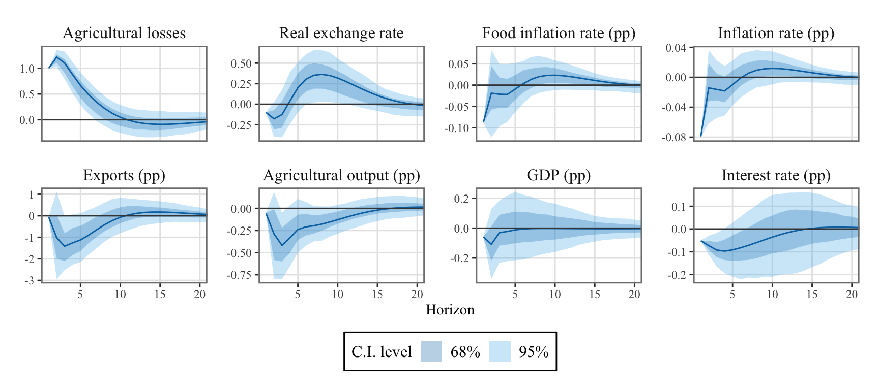
Figure 10.3: VAR(2) system response to one standard deviation orthogonal shock to the weather aggregate cost equation. The gray bands depict the 68% confidence intervals.

10.6 Estimation with Local Projections

We can also estimate the propagation of the shock using local projections rather than VAR.

Let us build the table with the data:

df_lp <- 
  df_var |> 
  filter(date >= start_date) |> 
  select(
    w, rer_dt_sa, pia, pi, x, q, y, r
  )

The linear impulse response functions can be estimated using the lp_lin() function from {lpirfs}.

library(lpirfs)
# With 95% conf. int.
results_lin_95 <- lp_lin(
  endog_data     = df_lp,
  lags_endog_lin = 2,# 2 lags
  trend          = 0,# no trend
  shock_type     = 0,# std dev. shock
  confint        = 1.96,
  hor            = 20
)
# With 68% conf. int.
results_lin_68 <- lp_lin(
  endog_data     = df_lp,
  lags_endog_lin = 2,# 2 lags
  trend          = 0,# no trend
  shock_type     = 0,# std dev. shock
  confint        = 1,
  hor            = 20
)

We define a small function, get_irfs(), to format the IRFs from the object returned by lp_lin().

get_irfs <- function(resul_lin) {
  irf_lin_mean <- resul_lin[["irf_lin_mean"]]
  irf_lin_low <- resul_lin[["irf_lin_low"]]
  irf_lin_up <- resul_lin[["irf_lin_up"]]
  specs <- resul_lin$specs
  
  irfs_df <- NULL
  for (rr in 1:(specs$endog)) {
    for (ss in 1:(specs$endog)) {
      tbl_lin_mean <- as.matrix(t(irf_lin_mean[, 1:specs$hor, ss]))[, rr]
      tbl_lin_low <- as.matrix(t(irf_lin_low[, 1:specs$hor, ss]))[, rr]
      tbl_lin_up <- as.matrix(t(irf_lin_up[, 1:specs$hor, ss]))[, rr]
      tbl_lin <- tibble(
        horizon = seq_along(tbl_lin_mean), 
        mean = tbl_lin_mean, 
        low = tbl_lin_low, 
        up = tbl_lin_up,
        shocked = specs$column_names[ss],
        on = specs$column_names[rr]
      )
      irfs_df <- bind_rows(irfs_df, tbl_lin)
    }
  }
  
  irfs_df <- 
    irfs_df |>
    mutate(
      shocked = factor(shocked, levels = variable_names, labels = names(variable_names)),
      on = factor(on, levels = variable_names, labels = names(variable_names))
    )
  
  irfs_df
}

The formatted IRFs:

irfs_df <- 
  get_irfs(results_lin_95) |> mutate(level = "95%") |> 
  bind_rows(
    get_irfs(results_lin_68) |> mutate(level = "68%")
  )

And the figure:

Code
ggplot() +
  geom_ribbon(
    data = irfs_df |> filter(shocked == "Agricultural losses"), 
    mapping = aes(
      x = horizon,
      ymin = low, ymax = up,
      fill = level),
    alpha = .3
  ) +
  geom_line(
    data = irfs_df |> filter(shocked == "Agricultural losses"), ,
    mapping = aes(x = horizon, y = mean),
    colour = "#0072B2"
  ) +
  geom_hline(yintercept = 0, colour = "#444444") +
  labs(x = "Horizon", y = NULL) +
  scale_fill_manual(
    "C.I. level", 
    values = c("68%" = "#0072B2", "95%" = "#56B4E9")) +
  facet_wrap(~on, scales = "free_y", ncol = 4) +
  theme_paper() +
  coord_cartesian(xlim = c(1, 20)) +
  scale_y_continuous(labels = scales::label_percent())
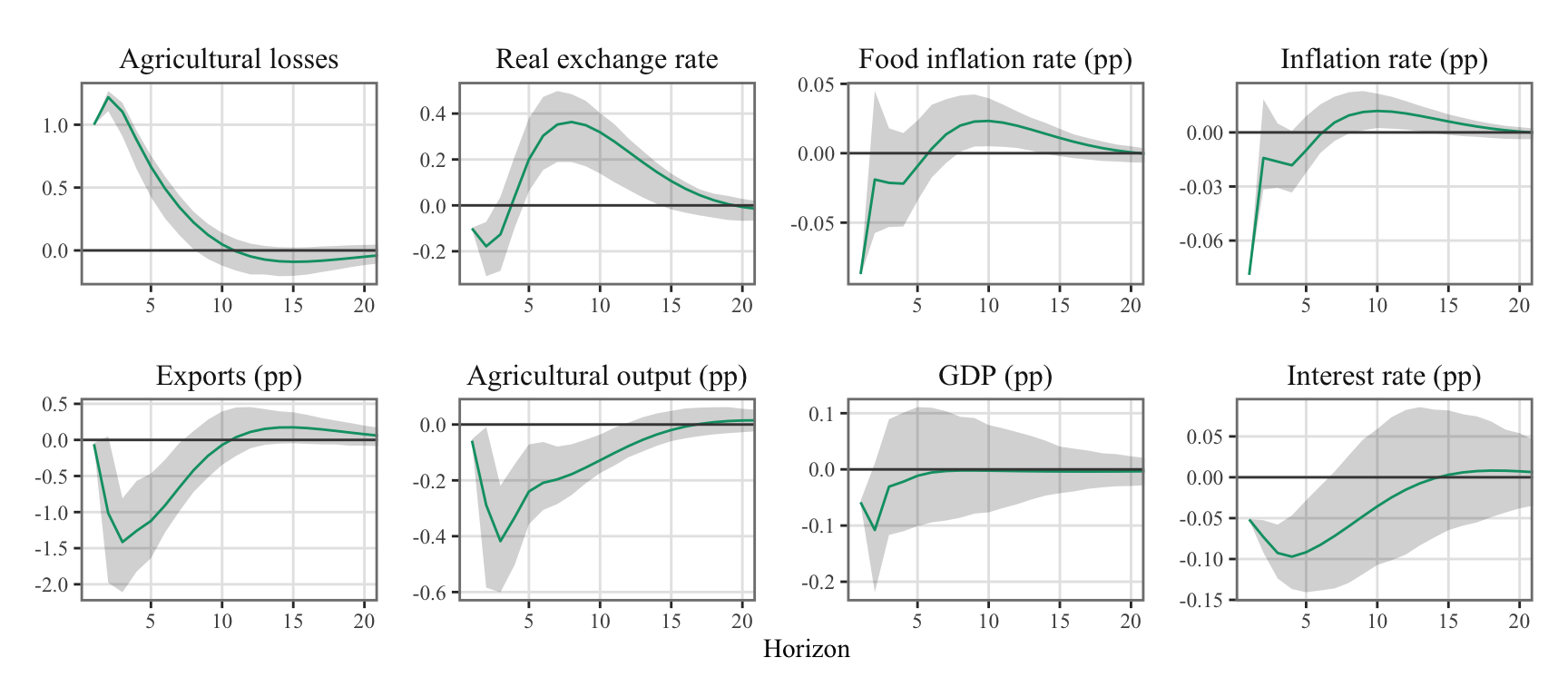
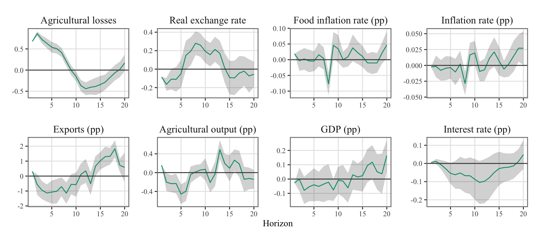
Figure 10.4: System response to one standard deviation orthogonal shock to the weather aggregate cost equation. Estimations made with local projections.

And with the 68% confidence interval only:

Code
library(tikzDevice)
library(lemon)
ggplot(
    data = irfs_df |> filter(shocked == "Agricultural losses") |> 
      filter(level == "68%") |> 
      mutate(level = str_replace(level, "\\%", "\\\\%")) |> 
      mutate(
        mean = mean * 100,
        low = low * 100,
        up = up * 100
      )
  ) +
  geom_ribbon(
    mapping = aes(x = horizon,ymin = low, ymax = up, fill = level),
    alpha = .2
  ) +
  geom_line(
    mapping = aes(x = horizon, y = mean),
    colour = "#009E73"
  ) +
  geom_hline(yintercept = 0, colour = "#444444") +
  labs(x = "Horizon", y = NULL) +
  scale_fill_manual(
    "C.I. level", 
    values = c("68\\%" = "gray10", "95\\%" = "gray60"),
    guide = "none") +
  facet_rep_wrap(~on, scales = "free_y", repeat.tick.labels = TRUE, ncol = 4) +
  theme_paper() +
  coord_cartesian(xlim = c(1, 20))
Figure 10.5: System response to one standard deviation orthogonal shock to the weather aggregate cost equation. Estimations made with local projections. The gray bands depict the 68% confidence intervals.

10.7 VAR vs LP

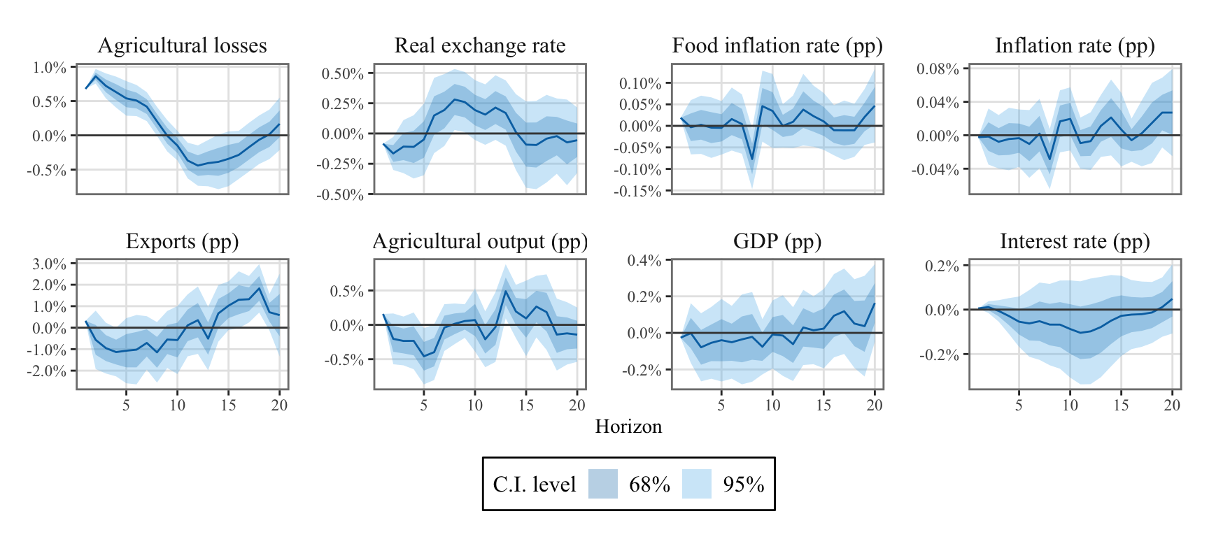
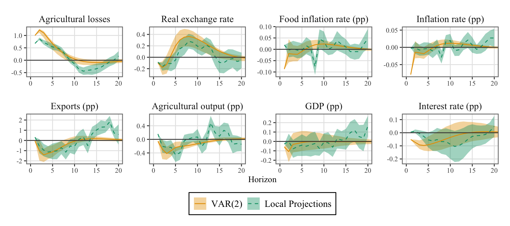
Let us graph the IRFs for both the VAR and the LPs on a single Figure.

Code
df_plot_comparison <- 
  df_irfs_ci |> 
  filter(level == "68%") |> 
  mutate(level = str_replace(level, "\\%", "\\\\%")) |> 
  mutate(estimation = "VAR(2)") |> 
  rename(on = name, shocked = impulse) |> 
  bind_rows(
    irfs_df |> filter(shocked == "Agricultural losses") |> 
      filter(level == "68%") |> 
      mutate(level = str_replace(level, "\\%", "\\\\%")) |> 
      mutate(
        mean = mean * 100,
        lower = low * 100,
        upper = up * 100
      ) |> 
      select(-low, -up) |> 
      mutate(estimation = "Local Projections")
  ) |> 
  mutate(
    estimation = factor(estimation, levels = c("VAR(2)", "Local Projections"))
  )

colour_1 <- "#E69F00"
colour_2 <- "#009E73"

p_comparison <- ggplot(
  data = df_plot_comparison
) +
  geom_ribbon(
    mapping = aes(x = horizon,ymin = lower, ymax = upper, fill = estimation),
    alpha = .4
  ) +
  geom_line(
    mapping = aes(x = horizon, y = mean, colour = estimation, linetype = estimation)
  ) +
  geom_hline(yintercept = 0, colour = "#444444") +
  labs(x = "Horizon", y = NULL) +
  scale_fill_manual(
    NULL,
    values = c("VAR(2)" = colour_1, "Local Projections" = colour_2)
  ) +
  scale_colour_manual(
    NULL,
    values = c("VAR(2)" = colour_1, "Local Projections" = colour_2)
  ) +
  scale_linetype_manual(
    NULL,
    values = c("VAR(2)" = "solid", "Local Projections" = "dashed")
  ) +
  facet_rep_wrap(~on, scales = "free_y", repeat.tick.labels = TRUE, ncol = 4) +
  theme_paper() +
  coord_cartesian(xlim = c(0, 20))
p_comparison
Figure 10.6: System response to one standard deviation orthogonal shock to the weather aggregate cost equation for VAR(2) and Local Projections frameworks. The bands depict the 68% confidence intervals.