15  Monthly/Quarterly/Annual Comparison (LP)

\[ \definecolor{bayesred}{RGB}{147, 30, 24} \definecolor{bayesblue}{RGB}{32, 35, 91} \definecolor{bayesorange}{RGB}{218, 120, 1} \definecolor{grey}{RGB}{128, 128, 128} \definecolor{couleur1}{RGB}{0,163,137} \definecolor{couleur2}{RGB}{255,124,0} \definecolor{couleur3}{RGB}{0, 110, 158} \definecolor{coul1}{RGB}{255,37,0} \definecolor{coul2}{RGB}{242,173,0} \definecolor{col_neg}{RGB}{155, 191, 221} \definecolor{col_pos}{RGB}{255, 128, 106} \definecolor{wongBlack}{RGB}{0,0,0} \definecolor{wongLightBlue}{RGB}{86, 180, 233} \definecolor{wongGold}{RGB}{230, 159, 0} \definecolor{wongGreen}{RGB}{0, 158, 115} \definecolor{wongYellow}{RGB}{240, 228, 66} \definecolor{wongBlue}{RGB}{0, 114, 178} \definecolor{wongOrange}{RGB}{213, 94, 0} \definecolor{wongPurple}{RGB}{204, 121, 167} \definecolor{IBMPurple}{RGB}{120, 94, 240} \definecolor{IBMMagenta}{RGB}{220, 38, 127} \]

Objectives

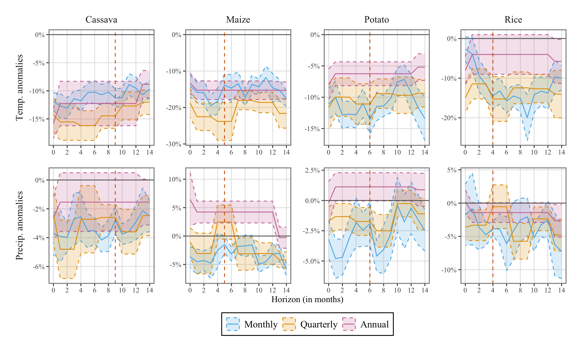
This chapter compares the response of agricultural production to a standard weather shock depending on the aggregation level of the agricultural data: monthly (as in Chapter 7), quarterly (Chapter 13), or annual (Chapter 14).

library(tidyverse)

── Attaching core tidyverse packages ──────────────────────── tidyverse 2.0.0 ──
✔ dplyr     1.1.4     ✔ readr     2.1.5
✔ forcats   1.0.0     ✔ stringr   1.5.1
✔ ggplot2   3.5.1     ✔ tibble    3.2.1
✔ lubridate 1.9.3     ✔ tidyr     1.3.1
✔ purrr     1.0.2     
── Conflicts ────────────────────────────────────────── tidyverse_conflicts() ──
✖ dplyr::filter() masks stats::filter()
✖ dplyr::lag()    masks stats::lag()
ℹ Use the conflicted package (<http://conflicted.r-lib.org/>) to force all conflicts to become errors

Let us load the theme function for graphs:

source("../weatherperu/R/utils.R")

Let us now load the estimations made in Chapter 7 with monthly production data:

load("../R/output/df_irfs_lp_piscop.rda")

Those made in Chapter 13 with quarterly production data:

load("../R/output/df_irfs_lp_quarter.rda")

And the estimations made in Chapter 14 with annual production data:

load("../R/output/df_irfs_lp_year.rda")

Let us merge the IRfs. We need to make sure that the values for each quarter are repeated 3 times so that the horizons can be compared. The same reasoning applies to annual data for which each year response is repeated 12 times.

df_irfs_lp_comparison <- df_irfs_lp |> 
  mutate(data_type = "monthly") |> 
  bind_rows(
    df_irfs_lp_quarter |> 
      mutate(data_type = "quarterly") |> 
      mutate(count = 3) |> 
      uncount(count) |> 
      group_by(crop, horizon, name) |> 
      mutate(
        horizon = ifelse(
          horizon != 0, 
          yes = (horizon-1)*3 + row_number(), no = 0
        )
      )
  ) |> 
  bind_rows(
    df_irfs_lp_year |> 
      mutate(data_type = "annual") |> 
      mutate(count = 12) |> 
      uncount(count) |> 
      group_by(crop, horizon, name) |> 
      mutate(
        horizon = ifelse(
          horizon != 0, 
          yes = (horizon-1)*12 + row_number(), no = 0
        )
      )
  ) |> 
  mutate(
    data_type = factor(
      data_type,
      levels = c("monthly", "quarterly", "annual"),
      labels = c("Monthly", "Quarterly", "Annual")
    )
  )

We do the same with confidence intervals:

df_irfs_lp_ci_comparison <- df_irfs_lp_ci |> 
  mutate(data_type = "monthly") |> 
  bind_rows(
    df_irfs_lp_ci_quarter |> 
      mutate(data_type = "quarterly") |> 
      mutate(count = 3) |> 
      uncount(count) |> 
      group_by(crop, horizon, name, level) |> 
      mutate(
        horizon = ifelse(
          horizon != 0, 
          yes = (horizon-1)*3 + row_number(), no = 0
        )
      )
  ) |> 
  bind_rows(
    df_irfs_lp_ci_year |> 
      mutate(data_type = "annual") |> 
      mutate(count = 12) |> 
      uncount(count) |> 
      group_by(crop, horizon, name, level) |> 
      mutate(
        horizon = ifelse(
          horizon != 0, 
          yes = (horizon-1)*12 + row_number(), no = 0
        )
      )
  ) |> 
  mutate(
    data_type = factor(
      data_type,
      levels = c("monthly", "quarterly", "annual"),
      labels = c("Monthly", "Quarterly", "Annual")
    )
  )

Then, we can plot the IRfs:

nb_h <- 14

# Duration of the growing season
gs_duration_df <- tribble(
  ~crop, ~tc,
  "Rice", 4,
  "Maize", 5,
  "Potato", 6,
  "Cassava", 9
)
ggplot() +
  geom_ribbon(
    data = df_irfs_lp_ci_comparison |> 
      filter(level == "68%", horizon <= !!nb_h),
    mapping = aes(
      x = horizon,
      ymin = lower, ymax = upper, fill = data_type, colour = data_type),
    alpha = .2, linetype = "dashed"
  ) +
  geom_line(
    data = df_irfs_lp_comparison |> filter(horizon <= !!nb_h),
    mapping = aes(x = horizon, y = shock_1_sd, colour = data_type)
  ) +
  scale_colour_manual(
    NULL, 
    values = c("Monthly" = "#56B4E9", "Quarterly" = "#E69F00", "Annual" = "#CC79A7")
  ) +
  geom_hline(yintercept = 0, colour = "gray40") +
  geom_vline(
    data = gs_duration_df, 
    mapping = aes(xintercept = tc),
    colour = "#D55E00", linetype = "dashed") +
  ggh4x::facet_grid2(
    name~crop, scales = "free_y", axes = "all",
    independent = "y", switch = "y") +
  scale_y_continuous(labels = scales::percent) +
  scale_x_continuous(breaks = seq(0, nb_h, by = 2)) +
  labs(x = "Horizon (in months)", y = NULL) +
  scale_fill_manual(
    NULL,
    values = c("Monthly" = "#56B4E9", "Quarterly" = "#E69F00", "Annual" = "#CC79A7")
  ) +
  theme_paper() +
  theme(strip.placement = "outside")

Figure 15.1: Agricultural production response to a weather shock, using either monthly, quarterly, or annual data.