16  Agricultural Production (LP)

Objectives

Estimate response functions of agricultural production following a weather shock, using Local Projections, with CHIRPS data instead of Piscop.

\[ \definecolor{bayesred}{RGB}{147, 30, 24} \definecolor{bayesblue}{RGB}{32, 35, 91} \definecolor{bayesorange}{RGB}{218, 120, 1} \definecolor{grey}{RGB}{128, 128, 128} \definecolor{couleur1}{RGB}{0,163,137} \definecolor{couleur2}{RGB}{255,124,0} \definecolor{couleur3}{RGB}{0, 110, 158} \definecolor{coul1}{RGB}{255,37,0} \definecolor{coul2}{RGB}{242,173,0} \definecolor{col_neg}{RGB}{155, 191, 221} \definecolor{col_pos}{RGB}{255, 128, 106} \definecolor{wongBlack}{RGB}{0,0,0} \definecolor{wongLightBlue}{RGB}{86, 180, 233} \definecolor{wongGold}{RGB}{230, 159, 0} \definecolor{wongGreen}{RGB}{0, 158, 115} \definecolor{wongYellow}{RGB}{240, 228, 66} \definecolor{wongBlue}{RGB}{0, 114, 178} \definecolor{wongOrange}{RGB}{213, 94, 0} \definecolor{wongPurple}{RGB}{204, 121, 167} \definecolor{IBMPurple}{RGB}{120, 94, 240} \definecolor{IBMMagenta}{RGB}{220, 38, 127} \]

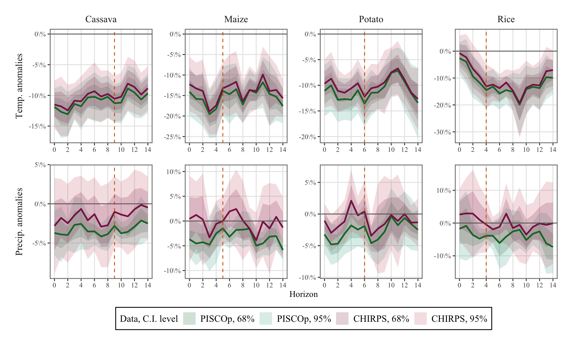
This chapter uses Jordà (2005) Local Projection framework to measure how sensitive agricultural output is to exogenous changes in the weather. It complements Chapter 7 and used CHIRPS precipitation data instead of Piscop.

library(tidyverse)
── Attaching core tidyverse packages ──────────────────────── tidyverse 2.0.0 ──
✔ dplyr     1.1.4     ✔ readr     2.1.5
✔ forcats   1.0.0     ✔ stringr   1.5.1
✔ ggplot2   3.5.1     ✔ tibble    3.2.1
✔ lubridate 1.9.3     ✔ tidyr     1.3.1
✔ purrr     1.0.2     
── Conflicts ────────────────────────────────────────── tidyverse_conflicts() ──
✖ dplyr::filter() masks stats::filter()
✖ dplyr::lag()    masks stats::lag()
ℹ Use the conflicted package (<http://conflicted.r-lib.org/>) to force all conflicts to become errors
library(fastDummies)
Thank you for using fastDummies!
To acknowledge our work, please cite the package:
Kaplan, J. & Schlegel, B. (2023). fastDummies: Fast Creation of Dummy (Binary) Columns and Rows from Categorical Variables. Version 1.7.1. URL: https://github.com/jacobkap/fastDummies, https://jacobkap.github.io/fastDummies/.

The data can be loaded (see Chapter 5)

load("../data/output/df_lp.rda")
df
# A tibble: 14,040 × 116
   product_eng region_id month date       y_new y_dev_pct y_new_normalized     y
   <chr>       <fct>     <dbl> <date>     <dbl>     <dbl>            <dbl> <dbl>
 1 Cassava     1             1 2001-01-01 5322     -0.452            0.548 0.527
 2 Cassava     1             2 2001-02-01 4388     -0.555            0.445 0.402
 3 Cassava     1             3 2001-03-01 5664.    -0.455            0.545 0.480
 4 Cassava     1             4 2001-04-01 5664.    -0.434            0.566 0.486
 5 Cassava     1             5 2001-05-01 5099     -0.534            0.466 0.370
 6 Cassava     1             6 2001-06-01 5537     -0.544            0.456 0.308
 7 Cassava     1             7 2001-07-01 5537     -0.523            0.477 0.335
 8 Cassava     1             8 2001-08-01 5993     -0.481            0.519 0.346
 9 Cassava     1             9 2001-09-01 5622.    -0.519            0.481 0.273
10 Cassava     1            10 2001-10-01 5622.    -0.464            0.536 0.315
# ℹ 14,030 more rows
# ℹ 108 more variables: t <int>, region <chr>, product <chr>, ln_prices <dbl>,
#   ln_produc <dbl>, year <dbl>, Value_prod <dbl>, surf_m <dbl>,
#   Value_surfR <dbl>, Value_prices <dbl>, campaign <dbl>,
#   campaign_plain <chr>, month_campaign <dbl>, surf_lag_calend <dbl>,
#   perc_product <dbl>, perc_product_mean <dbl>, diff_plant_harv <dbl>,
#   exposition <dbl>, exposition_trend <dbl>, exposition_detrended <dbl>, …

Some packages are needed, make sure that they are installed.

# install.packages("fastDummies")
# install.packages("imputeTS")
# install.packages("ggh4x")
# install.packages("mFilter")
# install.packages("pbapply")
# install.packages("latex2exp")
# install.packages("sandwich")

We load some useful functions:

# Functions useful to shape the data for local projections
source("../weatherperu/R/format_data.R")

# Load function in utils
source("../weatherperu/R/utils.R")

# Load detrending functions
source("../weatherperu/R/detrending.R")

16.1 Linear Local Projections

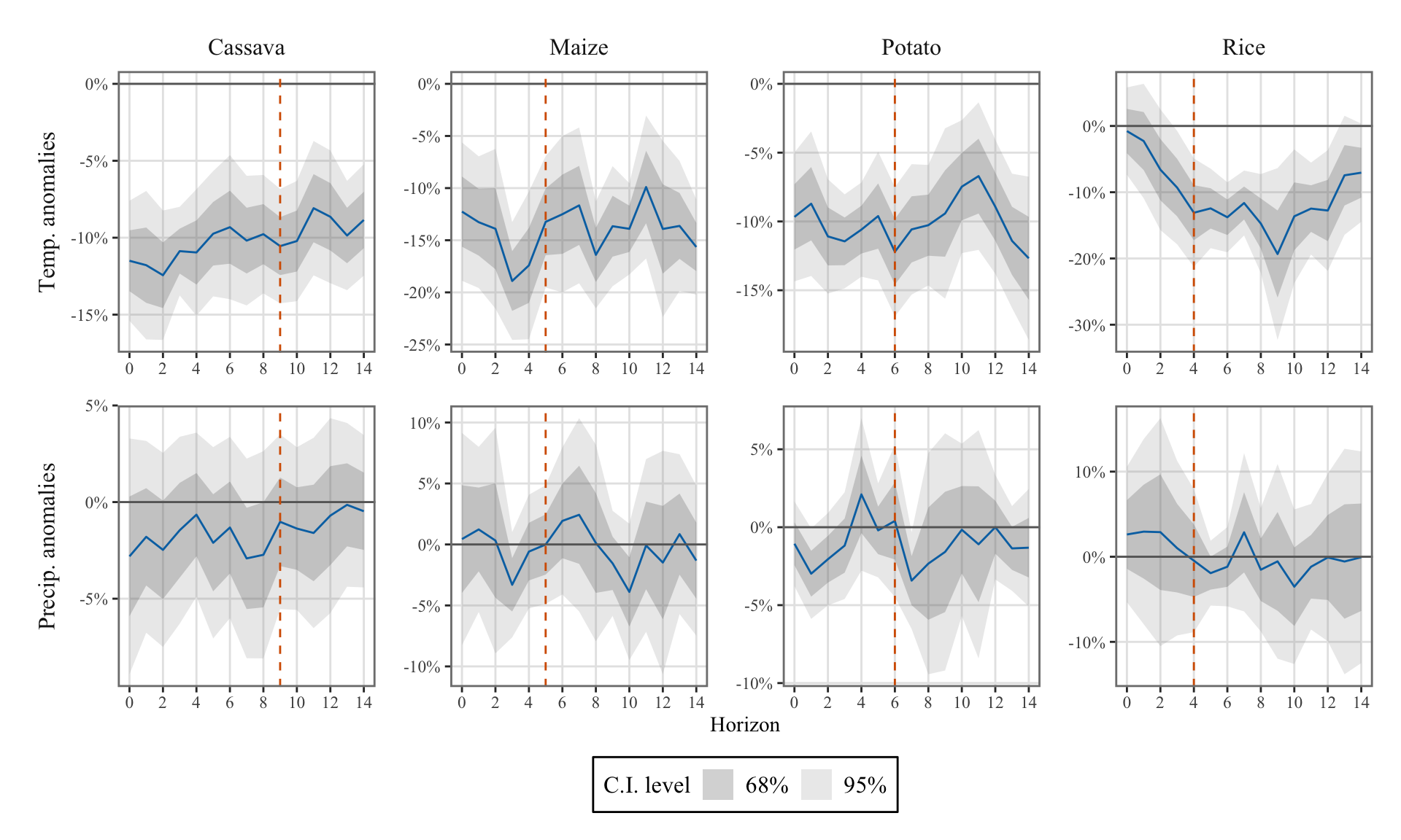
In this section, we focus on estimating the Local Projections (Jordà 2005) to quantify the impact of weather on agricultural production. We use panel data, similar to the approach used in the study by Acevedo et al. (2020), and independently estimate models for each specific crop.

For a particular crop denoted as \(c\), the model can be expressed as follows: \[ \begin{aligned} \underbrace{y_{c,i,{\color{wongGold}t+h}}}_{\text{Production}} = & {\color{wongOrange}\beta_{c,{\color{wongGold}h}}^{{\color{wongPurple}T}}} {\color{wongPurple}{T_{i,{\color{wongGold}t}}}} + {\color{wongOrange}\beta_{c,{\color{wongGold}h}}^{{\color{wongPurple}P}}} {\color{wongPurple}P_{i,{\color{wongGold}t}}}\\ &+\gamma_{c,i,h}\underbrace{X_{t}}_{\text{controls}} + \underbrace{\zeta_{c,i,h} \text{Trend}_{t} + \eta_{c,i,h} \text{Trend}^2_{t}}_{\text{regional monthly trend}} + \varepsilon_{c,i,t+h} \end{aligned} \tag{16.1}\]

Here, \(i\) represents the region, \(t\) represents the time, and \(h\) represents the horizon. The primary focus lies on estimating the coefficients associated with temperature and precipitation for different time horizons \(\color{wongGold}h=\{0,1,...,T_{c}\}\)

Note that we allow a crop regional monthly specific quadratic trend to be estimated.

16.1.1 Functions

The estimation functions presented in Chapter 7.1.1 can be sourced.

source("../weatherperu/R/estimations.R")

16.1.2 Estimation

To loop over the different crops, we can use the map() function. This function enables us to apply the estimate_linear_lp() function to each crop iteratively, facilitating the estimation process.

crops <- df$product_eng |> unique()
weather_variables <- c("temp_max_dev", "precip_sum_dev")
control_variables <- c(
  "rer_hp", "r_hp", "pi", "ind_prod", "ONI", "price_int_inf"
)
nb_h <- 14

The estimation (this code takes about a minute to run, we load results in this notebook):

resul_lp <- vector(mode = "list", length = length(crops))
for (i_crop in 1:length(crops)) {
  resul_lp[[i_crop]] <- estimate_linear_lp(
    df,
    horizons = nb_h,
    y_name = "y_new_normalized",
    group_name = "region_id",
    detrend = TRUE,
    add_month_fe = FALSE,
    add_intercept = FALSE,
    crop_name = crops[i_crop],
    control_names = control_variables,
    weather_names = weather_variables,
    std = "Cluster",
    # std = "nw",
    other_var_to_keep = "y_new"
  )
}
save(resul_lp, file = "..R/output/resul_lp_chirps.rda")
load("../R/output/resul_lp_chirps.rda")

16.1.3 Results

We can visualize the Impulse Response Functions (IRFs) by plotting the estimated coefficients associated with the weather variables. These coefficients represent the impact of weather on agricultural production and can provide valuable insights into the dynamics of the system. By plotting the IRFs, we can gain a better understanding of the relationship between weather variables and the response of agricultural production over time.

The data for the graphs:

df_irfs_lp <- map(resul_lp, "coefs") |> 
  list_rbind() |> 
  filter(name %in% weather_variables) |> 
  mutate(
    shock_1_sd = value * std_shock,
    lower_95 = (value - qnorm(0.975) * std) * std_shock,
    upper_95 = (value + qnorm(0.975) * std) * std_shock,
    lower_68 = (value - qnorm(0.84)  * std) * std_shock,
    upper_68 = (value + qnorm(0.84)  * std) * std_shock
  ) |> 
  mutate(
    crop = factor(
      crop, 
      levels = c("Rice", "Dent corn", "Potato", "Cassava"),
      labels = c("Rice", "Maize", "Potato", "Cassava"))
  ) |> 
  mutate(
    name = factor(
      name,
      levels = c(
        "temp_max_dev",
        "precip_sum_dev"
      ),
      labels = c(
        "Temp. anomalies", 
        "Precip. anomalies"
      )
    )
  )

For the confidence intervals:

df_irfs_lp_ci <- 
  df_irfs_lp |> 
  select(horizon, crop, name, matches("^(lower)|^(upper)", perl = TRUE)) |> 
  pivot_longer(
    cols = matches("^(lower)|^(upper)", perl = TRUE),
    names_pattern = "(.*)_(95|68)$",
    names_to = c(".value", "level")
  ) |> 
  mutate(level = str_c(level, "%"))
# Duration of the growing season
gs_duration_df <- tribble(
  ~crop, ~tc,
  "Rice", 4,
  "Maize", 5,
  "Potato", 6,
  "Cassava", 9
)
ggplot() +
  geom_ribbon(
    data = df_irfs_lp_ci |> filter(horizon <= !!nb_h),
    mapping = aes(
      x = horizon,
      ymin = lower, ymax = upper, fill = level),
    alpha = .2
  ) +
  geom_line(
    data = df_irfs_lp |> filter(horizon <= !!nb_h),
    mapping = aes(x = horizon, y = shock_1_sd),
    colour = "#0072B2") +
  geom_hline(yintercept = 0, colour = "gray40") +
  geom_vline(
    data = gs_duration_df, 
    mapping = aes(xintercept = tc),
    colour = "#D55E00", linetype = "dashed") +
  ggh4x::facet_grid2(
    name~crop, scales = "free_y", axes = "all",
    independent = "y", switch = "y") +
  scale_x_continuous(breaks = seq(0, nb_h, by = 2)) +
  scale_y_continuous(labels = scales::percent) +
  labs(x = "Horizon", y = NULL) +
  scale_fill_manual(
    "C.I. level", 
    values = c("68%" = "gray10", "95%" = "gray60")
  ) +
  theme_paper() +
  theme(strip.placement = "outside")
Figure 16.1: Agricultural production response to a weather shock

16.1.4 Exporting results

Let us save the results for later use.

save(df_irfs_lp, df_irfs_lp_ci, file = "../R/output/df_irfs_lp_piscop.rda")
save(resul_lp, file = "../R/output/resul_lp_piscop.rda")

16.2 Comparaison between PISCOp and CHIRPS

We can plot the IRFs obtained either using PISCOp or CHIRPS rainfall data.

Code
# With Piscop data
load("../R/output/df_irfs_lp_piscop.rda")
df_irfs_lp_piscop <- df_irfs_lp
df_irfs_lp_ci_piscop <- df_irfs_lp_ci
rm(df_irfs_lp, df_irfs_lp_ci)

# With Chirps data
load("../R/output/df_irfs_lp_chirps.rda")
df_irfs_lp_chirps <- df_irfs_lp
df_irfs_lp_ci_chirps <- df_irfs_lp_ci
rm(df_irfs_lp, df_irfs_lp_ci)

# Merge results
df_irfs_lp <- 
  df_irfs_lp_piscop |> mutate(data = "PISCOp") |> 
  bind_rows(df_irfs_lp_chirps |> mutate(data = "CHIRPS")) |> 
  mutate(data = factor(data, levels = c("PISCOp", "CHIRPS")))

df_irfs_lp_ci <- 
  df_irfs_lp_ci_piscop |> mutate(data = "PISCOp") |> 
  bind_rows(df_irfs_lp_ci_chirps |> mutate(data = "CHIRPS"))

# Aesthetics
df_irfs_lp_ci <- df_irfs_lp_ci |> 
  mutate(
    fill_lab = str_c(data, "_", level),
    fill_lab = factor(
      fill_lab, 
      levels = c("PISCOp_68%", "PISCOp_95%", "CHIRPS_68%", "CHIRPS_95%"), 
      labels = c("PISCOp, 68%", "PISCOp, 95%", "CHIRPS, 68%", "CHIRPS, 95%")
    )
  )
Code
ggplot() +
  geom_ribbon(
    data = df_irfs_lp_ci |> 
      filter(horizon <= !!nb_h),
    mapping = aes(
      x = horizon,
      ymin = lower, ymax = upper, fill = fill_lab),
    alpha = .2
  ) +
  geom_line(
    data = df_irfs_lp |> filter(horizon <= !!nb_h),
    mapping = aes(x = horizon, y = shock_1_sd, colour = data),
    linewidth = 1) +
  geom_hline(yintercept = 0, colour = "gray40") +
  geom_vline(
    data = gs_duration_df, 
    mapping = aes(xintercept = tc),
    colour = "#D55E00", linetype = "dashed") +
  ggh4x::facet_grid2(
    name~crop, scales = "free_y", axes = "all",
    independent = "y", switch = "y") +
  scale_x_continuous(breaks = seq(0, nb_h, by = 2)) +
  scale_y_continuous(labels = scales::label_percent(suffix = "\\%")) +
  labs(x = "Horizon", y = NULL) +
  scale_fill_manual(
    "Data, C.I. level", 
    values = c(
      "PISCOp, 68%" = "#117733", 
      "PISCOp, 95%" = "#44AA99", 
      "CHIRPS, 68%" = "#882255", 
      "CHIRPS, 95%" = "#CC6677"
    )
  ) +
  scale_colour_manual(
    NULL, values = c("PISCOp" = "#117733", "CHIRPS" = "#882255"), guide = "none"
  ) +
  theme_paper() +
  theme(strip.placement = "outside")
Figure 16.2: Agricultural production response to a weather shock, using PISCOp vs. CHIRPS data