4 Trees

This chapter presents some of the tree methods used for classification or regression problems. After presenting some data that will be used to illustrate the methods, it shows how decision trees work. Then, it present two ensemble methods based on decision trees: bagging and random forests. It is built using two main references: James et al. (2021), Boehmke and Greenwell (2019).

4.1 Data Used in the Notebook

To illustrate how to use tree-based methods, we will rely on Seoul bike sharing demand data set (Sathishkumar, Jangwoo, and Yongyun 2020 ; Sathishkumar and Yongyun 2020) freely available on the UCI Machine Learning Repository.

The data give the number of bicycles rented each hour from December 1st, 2017 to November 30th, 2018. It contains 8,760 observations. Some characteristics are made available on each day:

date: the date (day/month/year)
Rented Bike Count: number of bicycles rented
Hour: hour
Temperature(°C): temperature in Celcius degrees
Humidity(%): percentage of humidity
Wind speed (m/s): wind speed in metres per second
Visibility (10m): visibility at 10 metre
Dew point temperature(°C): dew point temperature in Celcius degrees, i.e., temperature to which air must be cooled to become saturated with water vapour
Solar Radiation (MJ/m2): solar radiation in megajoules per square metre
Rainfall(mm): rainfall in millimetres
Snowfall (cm): snowfall in centimetres
Seasons: season (Spring, Summer, Automn, Winter)
Holiday: holiday (Holiday, No Holiday)
Functioning Day: functioning day of the bicycle rental service (Yes, No)

We will need to use many functions from the packages of the tidyverse environment.

library(tidyverse)

A copy of the dataset is available on my website. The CSV file can directly be loaded in R as follows:

url <- "https://egallic.fr/Enseignement/ML/ECB/data/SeoulBikeData.csv"
bike <- read_csv(url, locale = locale(encoding = "latin1"))

There are a few days during which the rental service is not functioning:

table(bike$`Functioning Day`)

## 
##   No  Yes 
##  295 8465

For simplicity, let us remove the few observations for which the service is not functioning.

bike <- 
  bike %>% 
  filter(`Functioning Day` == "Yes") %>% 
  select(-`Functioning Day`)

The name of the variables is not convenient at all to work with. Let us rename the variables:

bike <- 
  bike %>% 
  rename(
    "date" = `Date`,
    "rented_bike_count" = `Rented Bike Count`,
    "hour" = `Hour`,
    "temperature" = `Temperature(°C)`,
    "humidity" = `Humidity(%)`,
    "wind_speed" = `Wind speed (m/s)`,
    "visibility" = `Visibility (10m)`,
    "dew_point_temperature" = `Dew point temperature(°C)`,
    "solar_radiation" = `Solar Radiation (MJ/m2)`,
    "rainfall" = `Rainfall(mm)`,
    "snowfall" = `Snowfall (cm)`,
    "seasons" = `Seasons`,
    "holiday" = `Holiday`
  )

There may be some seasonality in the data depending on: the hour, the day of the week, or the month of the year. While the hour is already given in the hour variable, the other component are not. Let us transform the date column in a date format. Then, the month and the day of the week can easily be extracted using functions from {lubidate}. We will provide the month name and the name of the week day in English. Depending on our settings, the functions month() and wday() from {lubridate} may give different outputs. We will thus make sure to set the time locale to English. The name of the locale is system dependent: on Unix, we can use "en_US", while on Windows, we can use "english_us".

loc_time_english <- 
  ifelse(.Platform$OS.type == "unix", "en_US", "english_us")

library(lubridate)

The new variables can be created as follows:

bike <- 
  bike %>% 
  mutate(
    date = dmy(date),
    year = year(date),
    month = month(date, label = TRUE, locale = loc_time_english),
    month = factor(as.character(month),
                   levels = c("Jan", "Feb", "Mar", "Apr", 
                              "May", "Jun", "Jul", "Aug", 
                              "Sep", "Oct", "Nov", "Dec")),
    week_day = wday(date, label = TRUE, locale = loc_time_english),
    week_day = factor(as.character(week_day),
                      levels = c("Mon", "Tue", "Wed", 
                                 "Thu", "Fri", "Sat", "Sun")),
    seasons = factor(seasons, levels = c("Spring", "Summer",
                                         "Autumn", "Winter"))
  )

Now, let us have a look at some summary statistics. First, we shall consider our target variable, i.e., the hourly number of bikes rented:

summary(bike$rented_bike_count)

##    Min. 1st Qu.  Median    Mean 3rd Qu.    Max. 
##     2.0   214.0   542.0   729.2  1084.0  3556.0

On average, there are 729 bikes rented per hour in Seoul over the considered period (December 2017 to November 2018).

We can have an idea of the distribution by plotting a histogram:

ggplot(data = bike, mapping = aes(x = rented_bike_count)) +
  geom_histogram(colour = "black") +
  labs(x = "Rented bike count", y = "Count")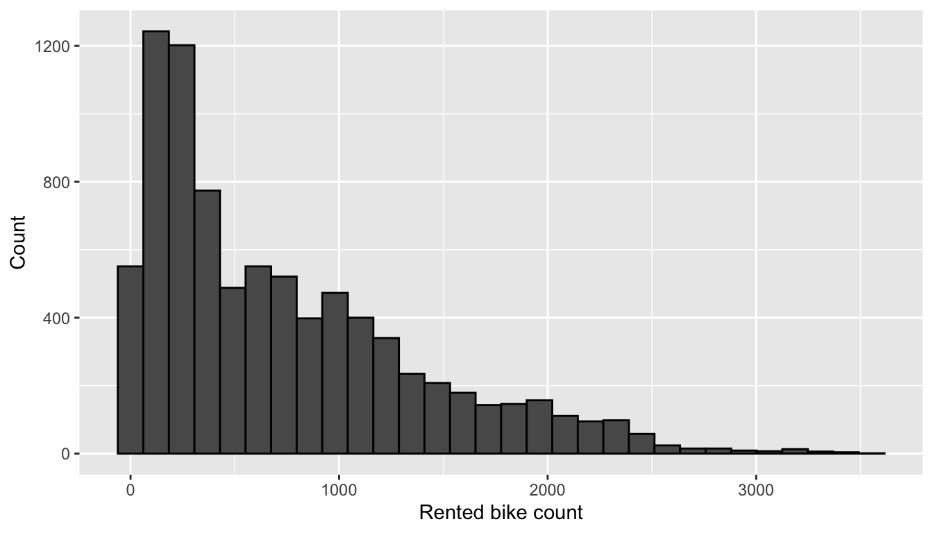

Figure 4.1: Distribution of rented bike count.

The distribution is skewed. Let us look at the distribution of the target variable depending on the month:

ggplot(data = bike, mapping = aes(x = rented_bike_count)) +
  geom_histogram(colour = "black") +
  labs(x = "Rented bike count", y = "Count") +
  facet_wrap(~month)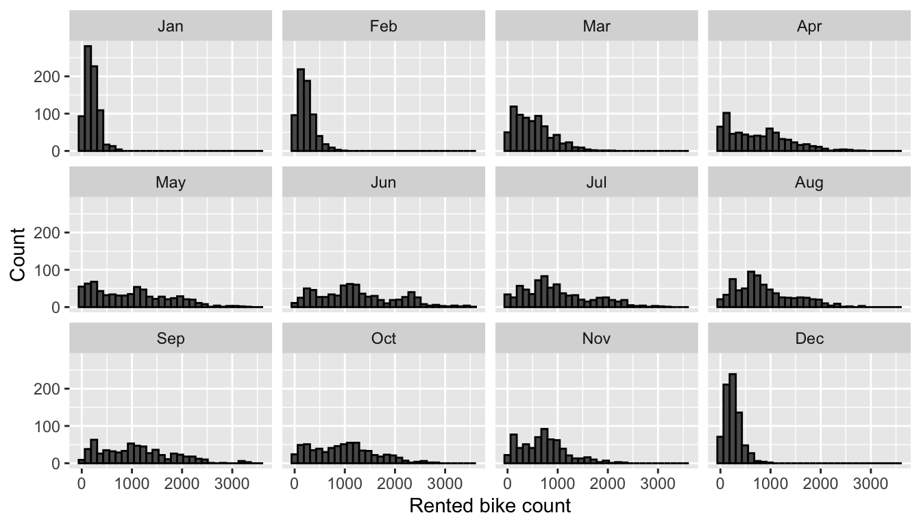

Figure 4.2: Distribution of rented bike count by month.

In cold months (December, January, February), the distribution appears to be concentrated around low values. There seems to be monthly seasonality here.

Let us look at the distribution of the number of bikes rented depending on the weekday:

ggplot(data = bike, mapping = aes(x = rented_bike_count)) +
  geom_histogram(colour = "black") +
  labs(x = "Rented bike count", y = "Count") +
  facet_wrap(~week_day)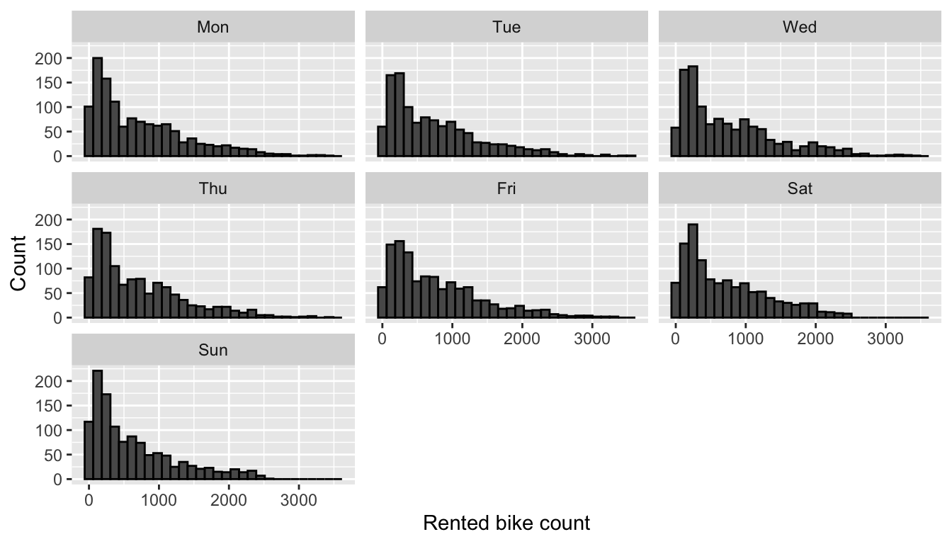

Figure 4.3: Distribution of rented bike count by weekday.

To the naked eye, there does not seem to be a specific link between the day of the week and the number of bicycles rented.

Somme summary statistics depending on the weekday can be obtained using the tableby() function from {arsenal}.

library(arsenal)
tableby_control <- tableby.control(
  numeric.stats=c("Nmiss", "meansd", "median", "q1q3")
)
tab <- tableby(week_day~rented_bike_count, data = bike, 
               control = tableby_control)
summary(tab, text = NULL) %>% 
  kableExtra::kable(
    caption = "Rented bike count depending on the week days.", booktabs = T,
    format = "latex", longtable = TRUE) %>%
  kableExtra::kable_classic(html_font = "Cambria") %>% 
  kableExtra::kable_styling(
    bootstrap_options = c("striped", "hover", "condensed",
                          "responsive", "scale_down"),
    font_size = 5)

The ANOVA test result reported in the previous table lead us to think that the mean is not the same across all weekdays. We notice that the number of rented bikes is relatively lower on Sundays and relatively higher on Fridays.

To have an idea of the distribution of the target variable conditional on the hour, we can use polar coordinates:

bike %>% 
  group_by(hour) %>% 
  summarise(rented_bike_count = mean(rented_bike_count)) %>% 
  ggplot(data = ., aes(x = hour, y = rented_bike_count)) +
  geom_bar(stat = "identity") +
  coord_polar() +
  labs(x = NULL, y = "Rented bike count") +
  scale_x_continuous(breaks = seq(0,24, by = 2))

Figure 4.4: Rented bike count per hour.

As one could expect, the number of bikes rented during the night are much lower that during the day. Two peaks are observed: around 8am and around 6pm, i.e., at the beginning and end of the working day.

We can also look at the distribution of the number of rented bikes depending on the seasons:

bike %>% 
  group_by(hour, seasons) %>% 
  summarise(rented_bike_count = mean(rented_bike_count)) %>% 
  ggplot(data = ., aes(x = hour, y = rented_bike_count)) +
  geom_bar(stat = "identity", mapping = aes(fill = seasons)) +
  coord_polar() +
  labs(x = NULL, y = "Rented bike count") +
  scale_x_continuous(breaks = seq(0,24, by = 2)) +
  facet_wrap(~seasons) +
  scale_fill_manual("Seasons", 
                    values = c("Spring" = "#004D40", "Summer" = "#FFC107",
                               "Autumn" = "#D81B60", "Winter" = "#1E88E5"))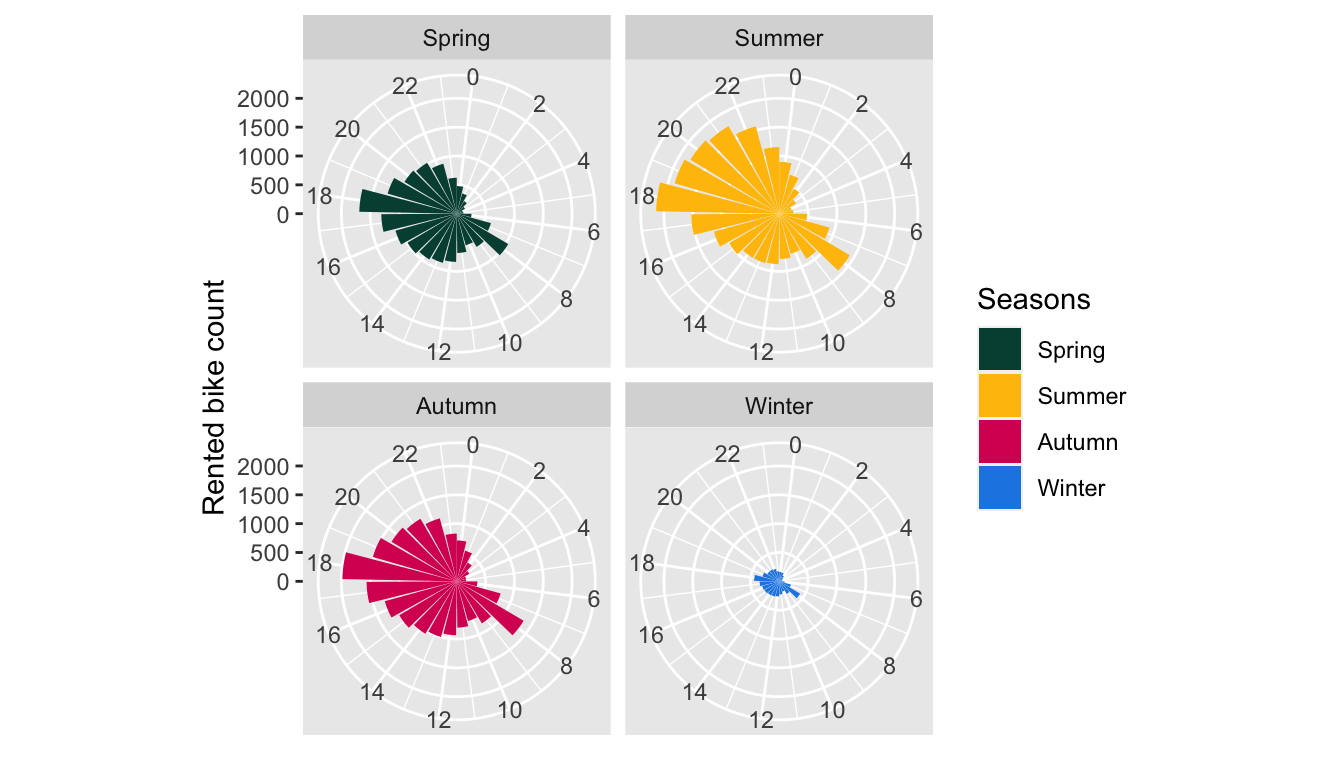

Figure 4.5: Rented bike count per hour and per season.

As previously seen, the number of rented bikes is much lower during Winter. The peaks at 8am and 6pm are observed regardless the seasons.

Now, using scatter plots, let us explore the relationship between the number of bikes rented and each weather variable. Let us first create each plot and store everyone of them in a different object.

library(cowplot)
p_temp <- 
  ggplot(data = bike, 
         mapping = aes(x = temperature, y = rented_bike_count)) +
  geom_point(alpha = .3) +
  geom_smooth() +
  labs(x = "Temperature (°C)", y = NULL,
       title = "Temperature vs humidity")

p_humidity <- 
  ggplot(data = bike, 
         mapping = aes(x = humidity, y = rented_bike_count)) +
  geom_point(alpha = .3) +
  geom_smooth() +
  labs(x = "Humidity (%)", y = NULL,
       title = "Rented count vs humidity")

p_wind <- 
  ggplot(data = bike, 
         mapping = aes(x = wind_speed, y = rented_bike_count)) +
  geom_point(alpha = .3) +
  geom_smooth() +
  labs(x = "Wind speed (m/s)", y = NULL,
       title = "Rented count vs wind speed")

p_visibility <- 
  ggplot(data = bike,
         mapping = aes(x = visibility, y = rented_bike_count)) +
  geom_point(alpha = .3) +
  geom_smooth() +
  labs(x = "Visibility (10m)", y = NULL,
       title = "Rented count vs visibility")

p_dew_point <- 
  ggplot(data = bike,
         mapping = aes(x = dew_point_temperature, y = rented_bike_count)) +
  geom_point(alpha = .3) +
  geom_smooth() +
  labs(x = "Dew point temperature (°C)", y = NULL,
       title = "Rented count vs dew point temperature")

p_solar_radiation <- 
  ggplot(data = bike, 
         mapping = aes(x = solar_radiation, y = rented_bike_count)) +
  geom_point(alpha = .3) +
  geom_smooth() +
  labs(x = "Solar Radiation (MJ/m2)", y = NULL,
       title = "Rented count vs solar radiation")


p_rainfall <- 
  ggplot(data = bike, 
         mapping = aes(x = rainfall, y = rented_bike_count)) +
  geom_point(alpha = .3) +
  geom_smooth() +
  labs(x = "Rainfall (mm)", y = NULL,
       title = "Rented count vs rainfall")

p_snowfall <- 
  ggplot(data = bike, 
         mapping = aes(x = snowfall, y = rented_bike_count)) +
  geom_point(alpha = .3) +
  geom_smooth() +
  labs(x = "Snowfall (cm)", y = NULL,
       title = "Rented count vs snowfall")

Then, using the plot_grid() function from {cowplot}, we can plot all these graphs on a single figure:

cowplot::plot_grid(p_temp, p_humidity, p_wind,
                   p_visibility, p_dew_point, p_rainfall,
                   p_snowfall, ncol = 2)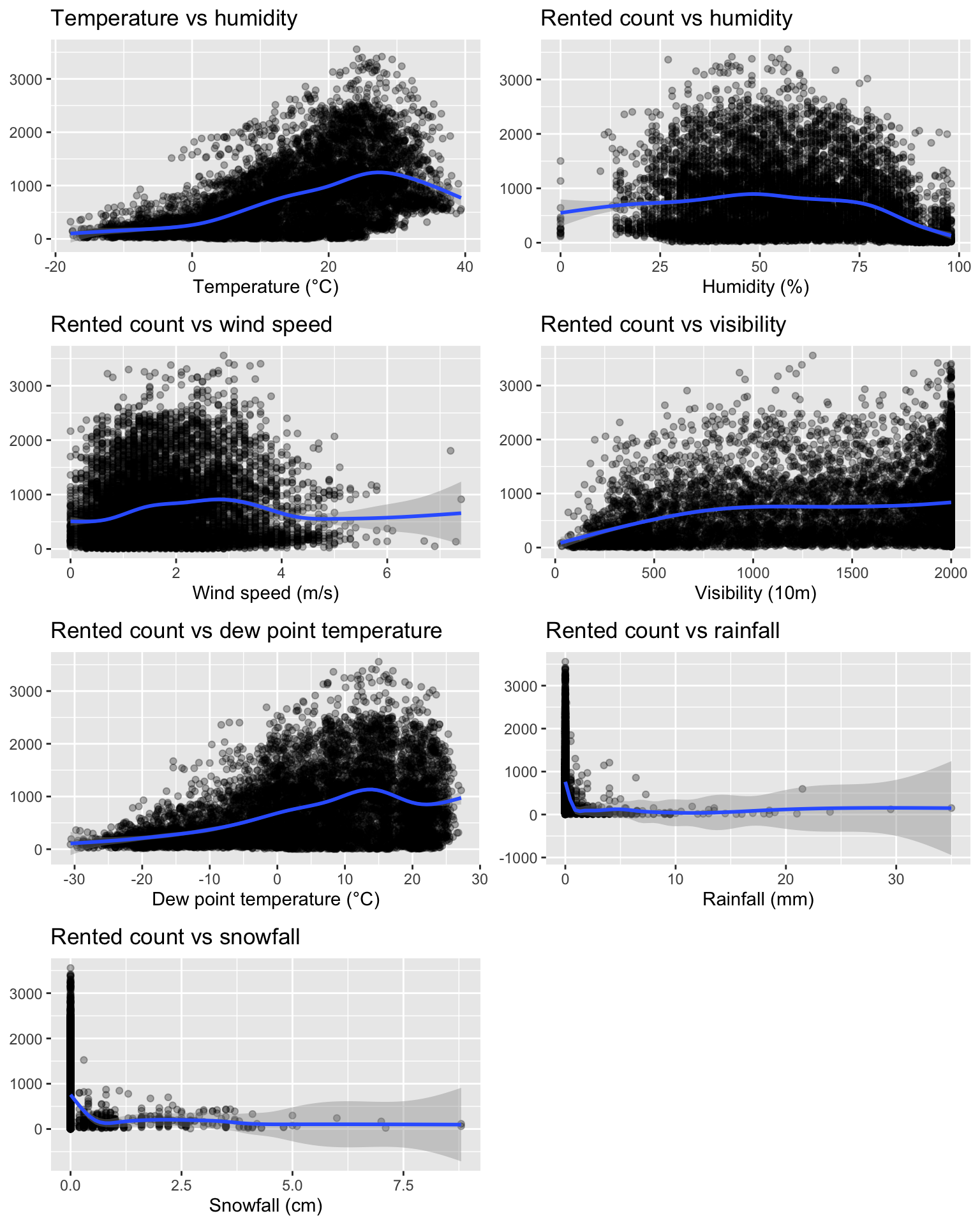

Figure 4.6: Relationship between the rented count and the numeric predictors.

The plot show nonlinear relationships between the weather and the number of rented bikes. One should note that these graphs do not allow to look at interaction effects.

Is there any correlation between the numerical variables of the dataset? Let us have a look.

correl_mat <- 
  bike %>% 
  select_if(is.numeric) %>% 
  cor() %>% 
  round(2)
correl_mat

##                       rented_bike_count  hour temperature humidity wind_speed
## rented_bike_count                  1.00  0.43        0.56    -0.20       0.13
## hour                               0.43  1.00        0.12    -0.24       0.29
## temperature                        0.56  0.12        1.00     0.17      -0.04
## humidity                          -0.20 -0.24        0.17     1.00      -0.34
## wind_speed                         0.13  0.29       -0.04    -0.34       1.00
## visibility                         0.21  0.10        0.03    -0.55       0.18
## dew_point_temperature              0.40  0.00        0.91     0.54      -0.18
##                       visibility dew_point_temperature solar_radiation rainfall
## rented_bike_count           0.21                  0.40            0.27    -0.13
## hour                        0.10                  0.00            0.14     0.01
## temperature                 0.03                  0.91            0.35     0.05
## humidity                   -0.55                  0.54           -0.46     0.24
## wind_speed                  0.18                 -0.18            0.33    -0.02
## visibility                  1.00                 -0.18            0.15    -0.17
## dew_point_temperature      -0.18                  1.00            0.10     0.13
##                       snowfall  year
## rented_bike_count        -0.15  0.23
## hour                     -0.02  0.00
## temperature              -0.22  0.38
## humidity                  0.11  0.04
## wind_speed                0.00  0.00
## visibility               -0.12  0.05
## dew_point_temperature    -0.15  0.33
##  [ getOption("max.print") est atteint -- 4 lignes omises ]

It may be more convenient to construct a correlation plot (we can do so here as the number of predictors is not too large).

library(corrplot)
corrplot.mixed(correl_mat, order = 'AOE')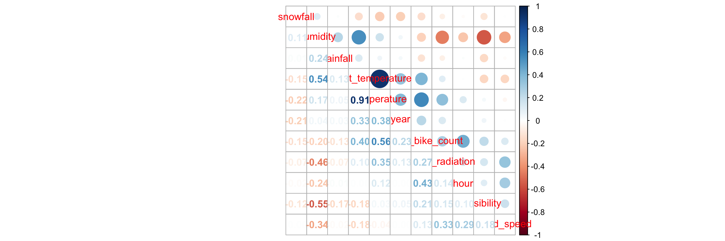

Figure 4.7: Correlation plot.

A nice summary table can also be constructed.

tableby_control <- tableby.control(
  numeric.stats=c("Nmiss", "meansd", "range", "median", "q1q3")
)
tab <- tableby(~., data = bike, control = tableby_control)
summary(tab, text = NULL) %>% 
  kableExtra::kable(caption = "Summary statistics.", booktabs = T,
                    format = "latex", longtable = TRUE) %>%
  kableExtra::kable_classic(full_width = F, html_font = "Cambria") %>% 
  kableExtra::kable_styling(
    bootstrap_options = c("striped", "hover", "condensed", "responsive"),
    font_size = 6)

For the sake of the illustration, let us create a binary outcome variable. Let us imagine that, for example, the service is too costly if the number of bikes rented per day is below 300. In such a case, we might want to train a classifier which will predict whether or not the number of bikes rented per day will be below or above that threshold.

bike <- 
  bike %>% 
  mutate(y_binary = ifelse(rented_bike_count < 300, "Low", "High"))

Let us look at the number and proportions of observations in each category:

table(bike$y_binary)

## 
## High  Low 
## 5526 2939

prop.table(table(bike$y_binary))

## 
##      High       Low 
## 0.6528057 0.3471943

We can also recreate the summary table depending on the binary outcome variable:

tableby_control <- tableby.control(
  numeric.stats=c("Nmiss", "meansd", "range", "median", "q1q3")
)
tab <- tableby(y_binary~., data = bike, control = tableby_control)
summary(tab, text = NULL) %>% 
  kableExtra::kable(
    caption = "Summary statistics depending on the binary response variable.", 
    booktabs = T,
    format = "latex", longtable = TRUE) %>%
  kableExtra::kable_classic(full_width = F, html_font = "Cambria") %>% 
  kableExtra::kable_styling(
    bootstrap_options = c("striped", "hover", "condensed", "responsive"),
    font_size = 6)

Now that we are a bit more familiar with the data, let us dig into the core subject of this notebook.

4.2 Training and Test Sets

Let us create a training dataset and a test dataset. We will put 80% of the first observations in the training set and the remaining 20% in the test set. Although we will not explore the time series aspect of the data at first, let us prepare the training and test sets such that the data in the test set will be those at the end of the sample period.

First, we need to make sure that the table is sorted by ascending values of date and then by ascending values of hour:

bike <- 
  bike %>% 
  arrange(date, hour)

Then the two sets can be created:

n_train <- round(.8*nrow(bike))

# Training set
df_train <- 
  bike %>% 
  slice(1:n_train)

# Test set
df_test <- 
  bike %>% 
  slice(-(1:n_train))

Let us look at the dimensions:

dim(df_train)

## [1] 6772   17

dim(df_test)

## [1] 1693   17

4.3 Decision Trees

In this first part, we will try to predict the number of rented bikes with a regression tree and then we will try to predict the binary outcome variable using a classification tree. The method we will used is called Classification and Regression Trees (CART) and was introduced in L. Breiman et al. (1984).

We will rely on {rpart} to build the tree and on {rpart.plot} to create graphical illustrations (whenever it is possible to do so).

library(rpart)
library(rpart.plot)

4.3.1 Regression Trees

To predict the number of hourly rented bikes, the predictor space will be segmented into a number of simple regions. To create these segments, the algorithm creates a series of binary splits. The data are recursively split into terminal nodes (leaves). Let us illustrate this with our data.

part_tree <- 
  rpart(rented_bike_count ~., 
        data = df_train %>% select(-y_binary, -date),
        method = "anova")

The rules that were learnt by the algorithm are the following

part_tree

## n= 6772 
## 
## node), split, n, deviance, yval
##       * denotes terminal node
## 
##   1) root 6772 2825639000  687.5492  
##     2) temperature< 12.15 3131  199783800  285.6675  
##       4) temperature< 5.65 2383   64996140  228.1637 *
##       5) temperature>=5.65 748  101804000  468.8650 *
##     3) temperature>=12.15 3641 1685319000 1033.1390  
##       6) hour< 15.5 2365  518621400  748.7455  
##        12) solar_radiation< 0.205 1084  114108200  460.0489  
##          24) hour>=1.5 801   61201670  362.2322 *
##          25) hour< 1.5 283   23550280  736.9081 *
##        13) solar_radiation>=0.205 1281  237713700  993.0445  
##          26) month=Mar,Apr,Jul,Aug 723   92311480  850.5007 *
##          27) month=May,Jun,Sep 558  111677400 1177.7380 *
##       7) hour>=15.5 1276  620889500 1560.2470  
##        14) rainfall>=0.05 109   19285900  259.2018 *
##        15) rainfall< 0.05 1167  399864100 1681.7670  
##          30) hour>=22.5 137   11867380 1124.7230 *
##          31) hour< 22.5 1030  339831500 1755.8590  
##            62) month=Mar,Apr,Aug 392   86211860 1483.6530 *
##            63) month=May,Jun,Jul,Sep 638  206727700 1923.1080  
##             126) humidity>=80.5 42   10854010 1015.6900 *
##             127) humidity< 80.5 596  158853500 1987.0540 *

They can be visualised using a tree:

rpart.plot(part_tree)

Figure 4.8: A first decision tree.

The first rule appears on top of the tree. Among all the tested separating rules, the one involving the variable temperature with a threshold of 12 is the one that minimises the residual sum of square (RSS). In other words, this couple of variable/cutoff value is the one that minimises deviations to the mean (variances) in each resulting leaf.

On the root node (top of the graph), the bubble shows two values:

688: this corresponds to the average value of the response variable for the observations in the node (here, the average for all observations)
100%: this percentage corresponds to the number of observation from the whole dataset that can be found in that node.

mean(df_train$rented_bike_count)

## [1] 687.5492

The first variable used to perform a split is temperature. Observations with a value for the variable temperature strictly lower than 12.15 (46%) will go to the left leaf. The others (the remaining 54%) will go to the right leaf.

Among the observations for which temperature is strictly lower than 12.15, the average of the response variable is equal to 286 (once rounded):

df_train %>% 
  filter(temperature < 12.15) %>% 
  summarise(mean = mean(rented_bike_count))

## # A tibble: 1 × 1
##    mean
##   <dbl>
## 1  286.

In that node, another split is performed, using the temperature variable once again, and the cutoff value that lead to the lowest RSS within that node is 5.65. Hence, observations for which the temperature is lower than 12.15 and lower than 5.65 (35% of all observations of the dataset) will go to the left leaf, while those for which the the temperature is lower than 12.15 and greater than 5.65 (11% of all observations of the dataset) will go to the right leaf.

df_train %>% 
  filter(temperature < 12.15) %>% 
  filter(temperature < 5.65) %>% 
  count() %>% 
  mutate(prop = n / nrow(df_train))

## # A tibble: 1 × 2
##       n  prop
##   <int> <dbl>
## 1  2383 0.352

We end up in a final node. The predicted value for such observations will be the average of the response variable in this node:

df_train %>% 
  filter(temperature < 12.15) %>% 
  filter(temperature < 5.65) %>% 
  summarise(pred = mean(rented_bike_count))

## # A tibble: 1 × 1
##    pred
##   <dbl>
## 1  228.

And on the right node:

df_train %>% 
  filter(temperature < 12.15) %>% 
  filter(temperature > 5.65) %>% 
  count() %>% 
  mutate(prop = n / nrow(df_train))

## # A tibble: 1 × 2
##       n  prop
##   <int> <dbl>
## 1   748 0.110

df_train %>% 
  filter(temperature < 12.15) %>% 
  filter(temperature > 5.65) %>% 
  summarise(pred = mean(rented_bike_count))

## # A tibble: 1 × 1
##    pred
##   <dbl>
## 1  469.

Let us detail the process of selecting the variable/cutoff pair. We can create a simple function to help compute the residual sum of squares:

compute_rss <- function(observed, predicted){
  sum((observed-predicted)^2)
}

Before making any split, the RSS is equal to:

rss_init <- 
  compute_rss(df_train$rented_bike_count, 
              mean(df_train$rented_bike_count))
rss_init

## [1] 2825639089

Let us consider the variable temperature used to partition the data, and a threshold of 12.15. Note that this variable is numerical. We will illustrate next how to procede with categorical data.

variable_split <- "temperature"
threshold <- 12.15

We split the data into two subsamples:

one for which temperature is below 12.15
another one for which temperature is greater than or equal to 12.15.

In each subset, we compute the average of the response variable: this will be the prediction made in the node:

tmp_data <- 
  df_train %>% 
  mutate(below_t = temperature < 12.15) %>% 
  select(rented_bike_count, below_t) %>% 
  group_by(below_t) %>% 
  mutate(pred = mean(rented_bike_count))

tmp_data

## # A tibble: 6,772 × 3
## # Groups:   below_t [2]
##    rented_bike_count below_t  pred
##                <dbl> <lgl>   <dbl>
##  1               254 TRUE     286.
##  2               204 TRUE     286.
##  3               173 TRUE     286.
##  4               107 TRUE     286.
##  5                78 TRUE     286.
##  6               100 TRUE     286.
##  7               181 TRUE     286.
##  8               460 TRUE     286.
##  9               930 TRUE     286.
## 10               490 TRUE     286.
## # … with 6,762 more rows

We can then compute the RSS :

rss_after_split <- 
  compute_rss(tmp_data$rented_bike_count, 
              tmp_data$pred)
rss_after_split

## [1] 1885102486

The improvement due to the split, in terms of percentage deviation of the RSS is given by:

-(rss_after_split - rss_init)/rss_init

## [1] 0.332858

It is the value reported in the split element of the object returned by rpart():

head(part_tree$splits)

##                       count ncat   improve index       adj
## temperature            6772   -1 0.3328580 12.15 0.0000000
## month                  6772   12 0.2719021  1.00 0.0000000
## seasons                6772    4 0.2395872  2.00 0.0000000
## dew_point_temperature  6772   -1 0.2132190  3.55 0.0000000
## hour                   6772   -1 0.1572311  6.50 0.0000000
## dew_point_temperature     0   -1 0.9162729  5.25 0.8189077

Now, let us wrap-up this code in a function, so that it is easy to make the threshold vary:

#' @param data data frame
#' @param variable_to_predict name of the variable to predict
#' @param variable_split name of the variable used to create the partitions
#' @param threshold threshold used to create the two partitions
rss_split_numeric <- 
  function(data, variable_to_predict, 
           variable_split, threshold){
    tmp_data <- 
      data %>% 
      mutate(below_t = !!sym(variable_split) < threshold) %>% 
      select(!!sym(variable_to_predict), below_t) %>% 
      group_by(below_t) %>% 
      mutate(pred = mean(!!sym(variable_to_predict)))
    
    compute_rss(tmp_data[[variable_to_predict]], tmp_data[["pred"]])
  }

An example with the same variable (temperature) and threshold (12.15) as earlier:

rss_split_numeric(
  data = df_train, variable_to_predict = "rented_bike_count",
  variable_split = "temperature", threshold = 12.15)

## [1] 1885102486

All that we need to to is to make the threshold vary. For example, we can consider values ranging from the minimum of the splitting variable to its maximum, so that 1000 different threshold values are tested:

number_of_cuts <- 1000
thresholds <- 
  seq(min(df_train$temperature), max(df_train$temperature),
      length.out = number_of_cuts)

Then, we can loop over these threshold values. At each iteration, we can store the RSS in a vector.

rss_tmp <- rep(NA, number_of_cuts)
for(i in 1:number_of_cuts){
  rss_tmp[i] <- 
    rss_split_numeric(
      data = df_train, variable_to_predict = "rented_bike_count",
      variable_split = "temperature", threshold = thresholds[i])
}

After a few seconds, once the loop has ended, we can look at the threshold value for which the RSS was the lowest:

thresholds[which.min(rss_tmp)]

## [1] 12.14555

We find the same value as that shown on top of the tree!

If we compute the average value of the number of rented bikes in each partition:

df_train %>% 
  mutate(below_t = temperature < thresholds[which.min(rss_tmp)]) %>% 
  select(rented_bike_count, below_t) %>% 
  group_by(below_t) %>% 
  summarise(pred = mean(rented_bike_count),
            n = n()) %>% 
  ungroup() %>% 
  mutate(prop = round(100*n/sum(n)))

## # A tibble: 2 × 4
##   below_t  pred     n  prop
##   <lgl>   <dbl> <int> <dbl>
## 1 FALSE   1033.  3641    54
## 2 TRUE     286.  3131    46

We get the values shown on top of the children nodes.

Then, we need to consider all variables as the variable used to partition the data (not only temperature). We will not do it here, but I am sure that you understood the process of selecting the splitting rule. What you may be now wondering, is how to proceed if the variable used to partition the data is not numerical, but categorical. In such a case, we just need to consider the combination of binary splits. For example, let us consider the variable month. There are $l=12$ months in the dataset, so that makes $2^{(l - 1)} - 1 = 2047$ possible binary splits:

(Jan) vs (Feb or Mar or Apr or May or Jun or Jul or Aug or Sep or Oct or Nov or Dec)
(Jan or Feb) vs (Mar or Apr or May or Jun or Jul or Aug or Sep or Oct or Nov or Dec)
(Jan or Mar) vs (Feb or Apr or May or Jun or Jul or Aug or Sep or Oct or Nov or Dec)
…
(Jan or Feb or Mar) vs (Apr or May or Jun or Jul or Aug or Sep or Oct or Nov or Dec)
…
(Jan or Feb or Mar or Apr or May or Jun or Jul or Aug or Sep or Oct or Nov) vs (Dec).

We can define a simple function that will give us all possible ways of creating unique binary partitions from a set of classes.

#' @param classes vector of names of classes
possible_splits <- function(classes){
  l <- length(classes)
  if(l>2){
    resul <- resul <- rep(NA, 2^(l-1) - 1)
    i <- 1
    for(k in 1:(l-1)){
      tmp <- combn(c(classes), k)
      for(j in 1:ncol(tmp)){
        if(tmp[1, j] != classes[1]) break
        current <- str_c(tmp[,j], collapse = ",")
        resul[i] <- str_c(tmp[,j], collapse = ",")
        i <- i+1
      }
    }
  }else{
    # If only two classes
    resul <- classes[1]
  }
  resul
}

This function just needs to be fed with a vector of classes. For example, if the classes are A, B, C, D, there will be $2^{(4 - 1)} - 1=7$ unique ways to partition the data into two areas.

possible_splits(c("A", "B", "C", "D"))

## [1] "A"     "A,B"   "A,C"   "A,D"   "A,B,C" "A,B,D" "A,C,D"

Let us illustrate how the partition is done on the tree by moving to one of the specific node: the one concerning observations for which temperature is greater than or equal to 12.15, the hour is lower than 15.5, the solar radiation is greater than or equal to 0.205.

Recall the plot:

rpart.plot(part_tree)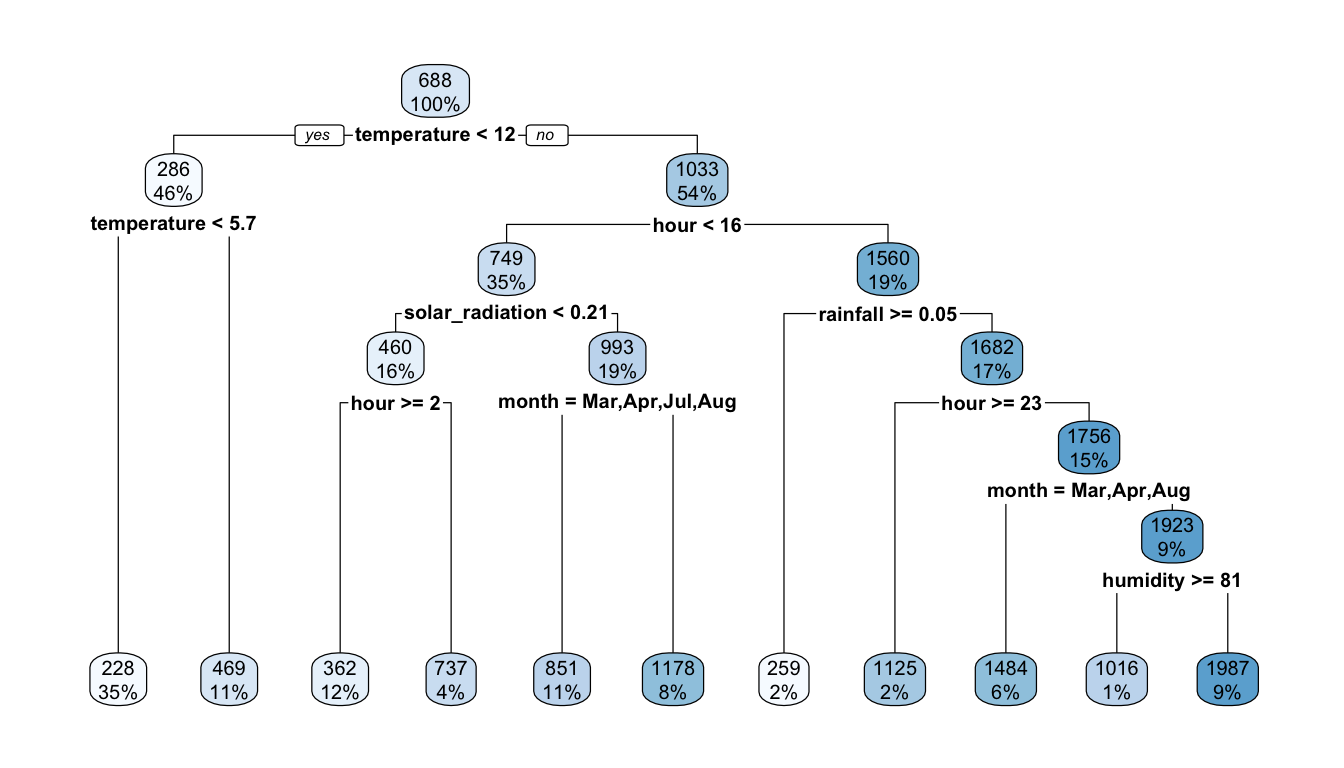

Figure 4.9: The same first decision tree.

df_tmp <- 
  df_train %>% 
  filter(temperature >= 12.15 & hour < 15.5 & solar_radiation >= 0.205)

The next partition, according to the graph, is done by separating observations for which the month is either March, April, July, or August from other observations. Let us try to retrieve such a result by hand.

At this node, we are left with 1281 observations:

nrow(df_tmp)

## [1] 1281

The different levels (or classes) of the month variable are the following:

classes <- as.character(unique(df_tmp$month))
classes

## [1] "Mar" "Apr" "May" "Jun" "Jul" "Aug" "Sep"

We note that there are less than 12 months in the dataset at this point. The number of classes is thus lower and the number of possible splits will thus be much smaller than 2047.

We can use our little function to obtain the list of possible splits:

list_possible_splits <- possible_splits(classes)
head(list_possible_splits)

## [1] "Mar"     "Mar,Apr" "Mar,May" "Mar,Jun" "Mar,Jul" "Mar,Aug"

There are actually 7 classes, so there are 63 possible splits:

length(list_possible_splits)

## [1] 63

Let us consider the following split:

list_possible_splits[2]

## [1] "Mar,Apr"

All we need to do is to create a variable that will state whether the month is either in March or in April, i.e., either in one of the elements of the following vector:

str_split(list_possible_splits[2], ",")[[1]]

## [1] "Mar" "Apr"

Then, we can group the observations by this dummy variable and compute the average of the response variable in each subset. This average will be the prediction made at this node, if we use (March or April) as the decision rule.

tmp_data <- 
  df_tmp %>% 
  mutate(var_in_categ = month %in% 
           str_split(list_possible_splits[2],",")[[1]])%>% 
  select(rented_bike_count, var_in_categ) %>% 
  group_by(var_in_categ) %>% 
  mutate(pred = mean(rented_bike_count))

We can check how many observations are in each subset:

table(tmp_data$var_in_categ)

## 
## FALSE  TRUE 
##  1065   216

And we need to compute the RSS:

compute_rss(tmp_data[["rented_bike_count"]], tmp_data[["pred"]])

## [1] 235207726

Now, let us wrap-up this in a function, so that it can be used over a loop where the decision rule is changed at each iteration:

#' @param data data frame
#' @param variable_to_predict name of the variable to predict
#' @param variable_split name of the variable used to create the partitions
#' @param split_rule vector of classes used to create the two partitions
rss_split_categ <- 
  function(data, variable_to_predict, 
           variable_split, split_rule){
    tmp_data <- 
      data %>% 
      mutate(var_in_categ = !!sym(variable_split) %in% split_rule) %>% 
      select(!!sym(variable_to_predict), var_in_categ) %>% 
      group_by(var_in_categ) %>% 
      mutate(pred = mean(!!sym(variable_to_predict)))
    
    compute_rss(tmp_data[[variable_to_predict]], tmp_data[["pred"]])
  }

With the same rule as that used in the example, the function rss_split_categ() can be used as follows:

rss_split_categ(df_tmp, 
                variable_to_predict = "rented_bike_count",
                variable_split = "month", 
                split_rule = str_split(list_possible_splits[2], ",")[[1]])

## [1] 235207726

Let us loop over all the possible splits, and store the RSS at each iteration.

rss_tmp <- rep(NA, length(list_possible_splits))
for(i in 1:length(list_possible_splits)){
  rss_tmp[i] <- 
    rss_split_categ(
      df_tmp, 
      variable_to_predict = "rented_bike_count",
      variable_split = "month", 
      split_rule = str_split(list_possible_splits[i], ",")[[1]])
}

The RSS is at its lowest for this variable with the following rule:

list_possible_splits[which.min(rss_tmp)]

## [1] "Mar,Apr,Jul,Aug"

Good news, we obtain the same result as that provided by the rpart() function! We can also check that the predictions in each subset and the proportion of observations are the same as that obtained with rpart().

df_tmp %>% 
  mutate(var_in_categ = month %in% 
           str_split(list_possible_splits[which.min(rss_tmp)],",")[[1]])%>% 
  select(rented_bike_count, var_in_categ) %>% 
  group_by(var_in_categ) %>% 
  summarise(pred = mean(rented_bike_count),
            n = n()) %>% 
  mutate(prop = round(100*n/nrow(df_train)))

## # A tibble: 2 × 4
##   var_in_categ  pred     n  prop
##   <lgl>        <dbl> <int> <dbl>
## 1 FALSE        1178.   558     8
## 2 TRUE          851.   723    11

rpart.plot(part_tree)

Figure 4.10: The same (again) first decision tree.

To sum up, at each node, each variable is tested as a candidate to segment the input space into two parts. Multiple splits are tested for each variables. The final choice is the variable and the splitting rule leading to the lowest RSS value.

Once a split is done, the splitting process can be repeated in each partition. This process goes on recursively until some stopping criteria. All the variables are again considered as candidates, even the one that was used in the previous split.

4.3.2 Stopping the Recursive Splitting Process

The question that can then be asked is: what criteria should be used to decide to stop the recursive partitioning process?

There are multiple ways of stopping the algorithm. These ways are controlled by the arguments of the function rpart.control() from {rpart}. Some of them are the following:

maxdepth: we can set the maximum depth of the tree, with the root node counted as depth 0
minsplit: we can decide that in order to make a split, there should be at least a minimum number of observations in a node ; if it is not the case, the split should not be attempted
minbucket: we can also decide that a split should not be performed if it leads to a leaf node with too few observations (by default, this value is set in R as 1/3 of minsplit)
cp: in the case of regression trees with anova splitting, if the split leads to an increase in the R-squared less than cp compared to the previous value, then the split should not be done. Setting cp=0 will lead to overlooking this criterion as a stopping criterion.

These arguments can be directly provided to the rpart() function. In the following example, a split will be attempted if there is at least 1,000 observation in the node for which the split is performed, and if it leads to partitions in which at least 500 observations are left in the leaf node. If attempting the split respects these two conditions, we will overlook the fact that the R-squared should be increased at the next step, by setting cp=-1.

part_tree <- 
  rpart(rented_bike_count ~., 
        data = df_train %>% select(-y_binary, -date),
        method = "anova",
        minsplit = 1000,
        minbucket = 500,
        cp=0)
rpart.plot(part_tree)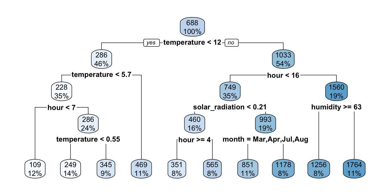

Decision tree where splits are made if there is at least 1000 obs. in the node and if the number of obs. in the resulting leaves are at least 500.

Figure 4.11: Decision tree where splits are made if there is at least 1000 obs. in the node and if the number of obs. in the resulting leaves are at least 500.

If now we allow splits to be done with the same conditions but only if they lead to an increase in the R-squared value of 0.01 from one step to the next:

part_tree <- 
  rpart(rented_bike_count ~., 
        data = df_train %>% select(-y_binary, -date),
        method = "anova",
        minsplit = 1000,
        minbucket = 500,
        cp=.01)
rpart.plot(part_tree)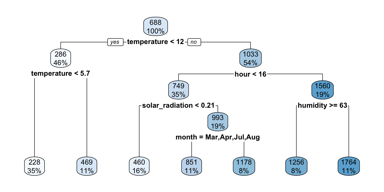

Figure 4.12: Growing the tree stopped earlier as we imposed restrictions on the improvement needed to make split.

It can be noted that the tree is a bit shallower.

The tree grown has a depth of 4. Let us constrain the tree to have a maximum depth of only 3.

part_tree <- 
  rpart(rented_bike_count ~., 
        data = df_train %>% select(-y_binary, -date),
        method = "anova",
        maxdepth = 3,
        cp = 0)
rpart.plot(part_tree)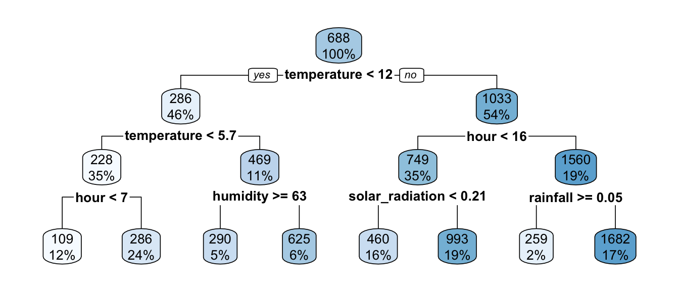

Figure 4.13: Decision tree when constraining its depth.

The algorithm stopped earlier.

Let us spent a bit more time with the two parameters controlling the maximum depth of the tree and the minimum number of observations in a node for a split to be attempted. We can easily give the intuition that the higher the depth of the tree, the higher the risk of overfitting. In a same way, the lower the minimum number of observations in a node for a split to be attempted, the higher the risk of overfitting. Let us give an illustration with synthetic data. Let us assume that we observe 100 observations drawn from the following process:

\[y_i= .1x_i^3 -x_i^2+x_i + \varepsilon_i, \quad \varepsilon \sim \mathcal{N}(0,4).\]

set.seed(123)
n <- 100
x <- runif(n=n, min=0, max=10)
eps <- rnorm(n, 0, 4)
f <- function(x) .1*x^3-1*x^2+x
y <- f(x)+eps

Let us plot the observed values and show with a red dotted line the expected value of data drawn from this data generating process.

df_sim <- tibble(x=x, y=y)
ggplot(data = df_sim, mapping = aes(x = x, y = y)) +
  geom_line(data = tibble(x=seq(0, 10, by = .1), y=f(x)),
            size = 1.1, linetype = "dashed", colour = "#AA2F2F") +
  geom_point()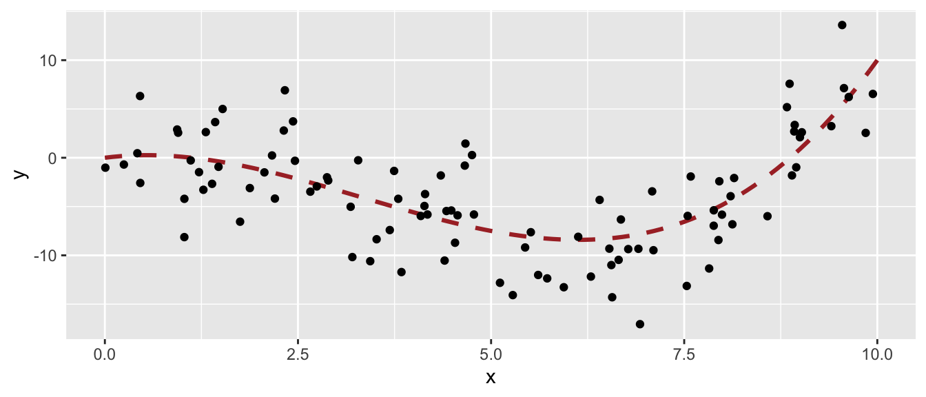

Figure 4.14: Generating Data Process and generated data.

Now, let us train a regression tree on the observed values. Let us limit the depth of the tree to 1.

part_tree <- 
  rpart(y ~ x, 
        data = df_sim,
        method = "anova",
        maxdepth = 1,
        cp = 0
  )
rpart.plot(part_tree)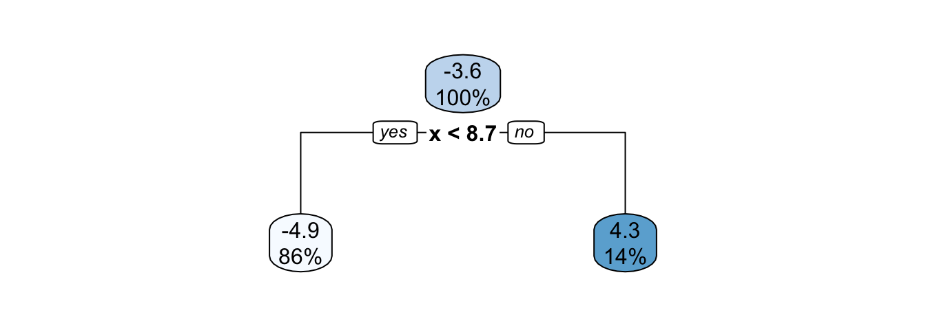

Figure 4.15: Decision tree built on the synthetic data with a maximum depth of 1.

The decision boundary is such that if x is lower than 8.7, the predicted value will be -4.9; otherwise it will be 4.3.

ggplot(mapping = aes(x = x, y = y)) +
  geom_line(data = tibble(x=seq(0, 10, by = .1), y=f(x)),
            size = 1.1, linetype = "dashed", colour = "#AA2F2F") +
  geom_point(data = df_sim) +
  geom_segment(data = tibble(x = c(-Inf, 8.7), 
                             xend = c(8.7, Inf),
                             y = c(-4.9, 4.3), 
                             yend = c(-4.9, 4.3)),
               mapping = aes(x=x, y=y, xend=xend, yend=yend),
               colour = "#005A8B", size = 1.5)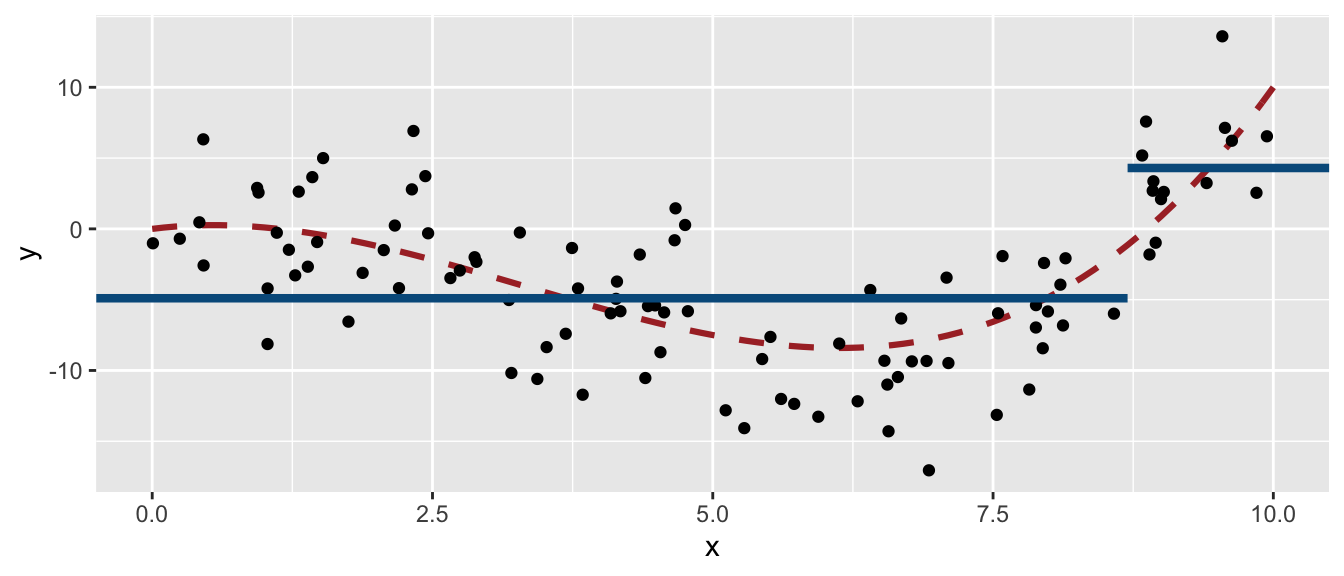

Figure 4.16: Decision boundary of the grown tree.

Now let us vary the maxdepth and minsplit parameters over a loop. We can create a function that will return the decision boundaries (to be precise, it is not exactly the exact decision boundaries that is returned, but a very close approximation).

get_pred_part <- function(max_depth, min_split){
  part_tree <- 
    rpart(y ~ x, 
          data = df_sim,
          method = "anova",
          minsplit = min_split,
          maxdepth = max_depth,
          cp = 0
    )
  
  tibble(
    x = seq(0, 10, by = .1),
    y = predict(part_tree, newdata = tibble(x=seq(0, 10, by = .1))),
    max_depth = max_depth,
    min_split = min_split
  )
  
}

We will loop over all the combinations that can be made up with the values for maxdepth and minsplit that we define, and apply the get_pred_part() at each iteration.

predicted_vals <- 
  list(
    max_depth = c(1, 3, 5, 10),
    min_split = c(2, 10, 20)) %>% 
  cross() %>% 
  map_df(purrr::lift(get_pred_part))
predicted_vals

## # A tibble: 1,212 × 4
##        x     y max_depth min_split
##    <dbl> <dbl>     <dbl>     <dbl>
##  1   0   -4.92         1         2
##  2   0.1 -4.92         1         2
##  3   0.2 -4.92         1         2
##  4   0.3 -4.92         1         2
##  5   0.4 -4.92         1         2
##  6   0.5 -4.92         1         2
##  7   0.6 -4.92         1         2
##  8   0.7 -4.92         1         2
##  9   0.8 -4.92         1         2
## 10   0.9 -4.92         1         2
## # … with 1,202 more rows

library(ggtext)
ggplot(mapping = aes(x = x, y = y)) +
  geom_line(data = tibble(x=seq(0, 10, by = .1), y=f(x)),
            size = 1.1, linetype = "dashed", colour = "#AA2F2F") +
  geom_point(data = df_sim) +
  geom_step(data = predicted_vals %>% 
              mutate(max_depth = factor(
                max_depth, 
                levels = sort(unique(predicted_vals$max_depth)),
                labels = str_c("Max depth: ", 
                               sort(unique(predicted_vals$max_depth)))),
                min_split = factor(
                  min_split, 
                  levels = sort(unique(predicted_vals$min_split), 
                                decreasing = TRUE),
                  labels = str_c("Min node size: ", 
                                 sort(unique(predicted_vals$min_split), 
                                      decreasing = TRUE)))
              ),
            colour = "#005A8B", size = 1.5) +
  facet_grid(max_depth~min_split) +
  labs(title = str_c(
    "Change in **<span style='color:#005A8B'>",
    "decision boundaries</span>** induced by parameter variations")
  ) +
  theme(
    plot.title = element_markdown(lineheight = 1.1),
    plot.title.position = "plot",
    legend.text = element_markdown(size = 11)
  )

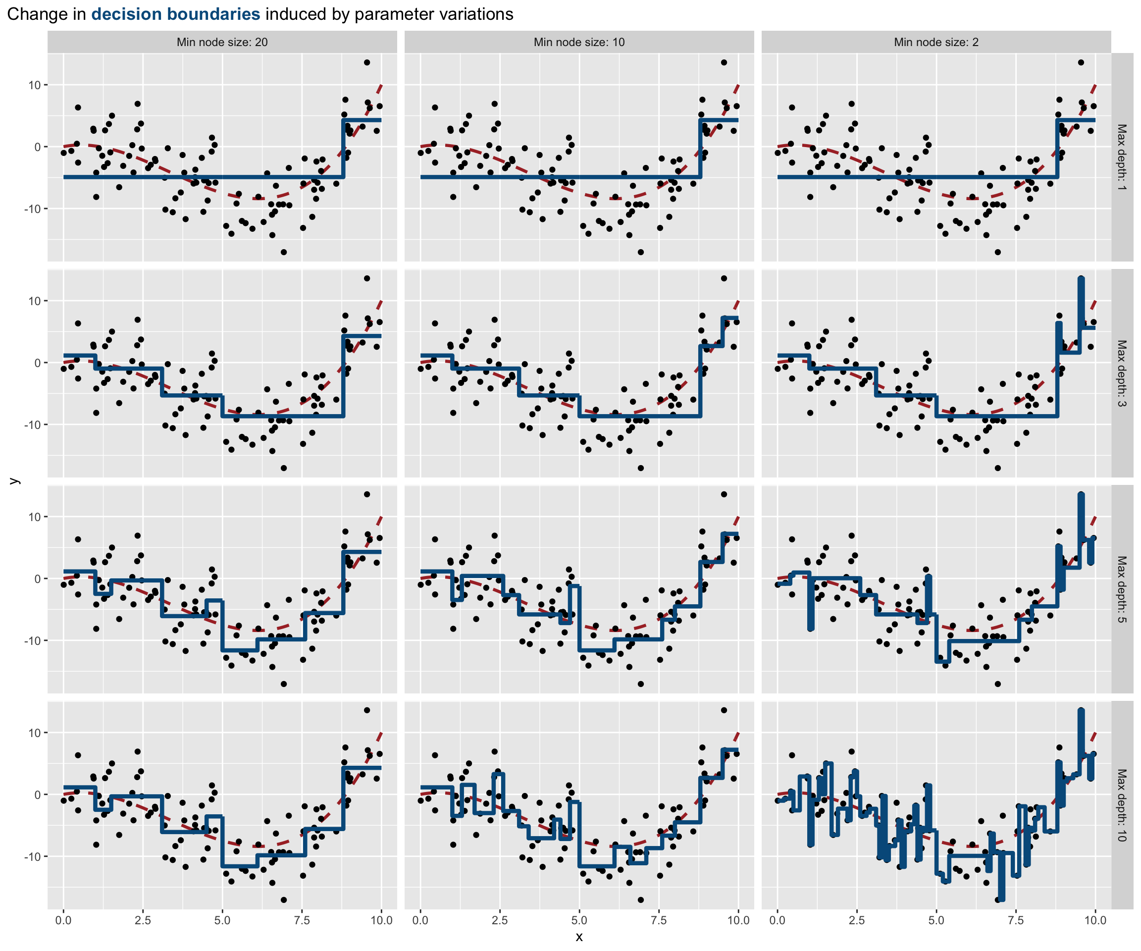
Figure 4.17: Varying the parameters affect the decision boundary and may lead to overfitting.

In the previous graph, we clearly note that:

if the maximum depth of the tree that is grown is 1, then the minimum node size does not play any role
as long as we increase the maximum depth, the boundary decision gets closer to the points: there is a risk of overfitting
as long as the number of minimum observations in a node for a split to be attempted decreases, the boundary decision gets closer to the points: there is once again a risk of overfitting.

4.3.2.1 Pruning

With the previous example, we saw that smaller trees lead to lower variance. They also lead to better interpretation. On the other hand, this is done at the expense of a little bias. We might be tempted to rely on growing small trees, by stropping the algorithm as soon as the decrease in the SSR due to the current split falls below some threshold. But this is too short-sided, as a poor split could be followed by a very good split.

Another strategy, called tree pruning, consists in growing a large tree, and then prune it back to keep only a subtree. To determine the level at which pruning is carried out, we can proceed by cross-validation. But instead of considering all trees, only a subset of those are considered. The cross-validation process is used to select a penalization parameter ($\lambda$). As explained in Emmanuel Flachaire’s course, we put a prize to pay for having a tree with many terminal nodes $J$, or regions,

\[\min \sum_{j=1}^{J} \sum_{i \in R_j}(y_i-\overline{y}_{R_j})^2+ \lambda J.\]

With a value of $\lambda=0$, the subtree we end up with is the large tree we grew in the first place. As long as we increase the value of $\lambda$, having many terminal nodes $J$ become costlier.

In {rpart}, the number of folds for the cross-validation is provided through the xval argument of the rpart.control() function. It can also be given directly to the rpart() function.

Let us perform a 10-fold cross validation with the Seoul bike data (this is actually done by default when calling the rpart() function).

set.seed(123)
large_tree <- 
  rpart(rented_bike_count ~., 
        data = df_train %>% select(-y_binary, -date),
        method = "anova",
        control = rpart.control(xval = 10, cp = -1, minbucket = 20))

# Number of nodes
nodes_large_tree <- as.numeric(rownames(large_tree$frame))
max(rpart:::tree.depth(nodes_large_tree))

## [1] 16

We can plot the results of the cross-validation:

plotcp(large_tree)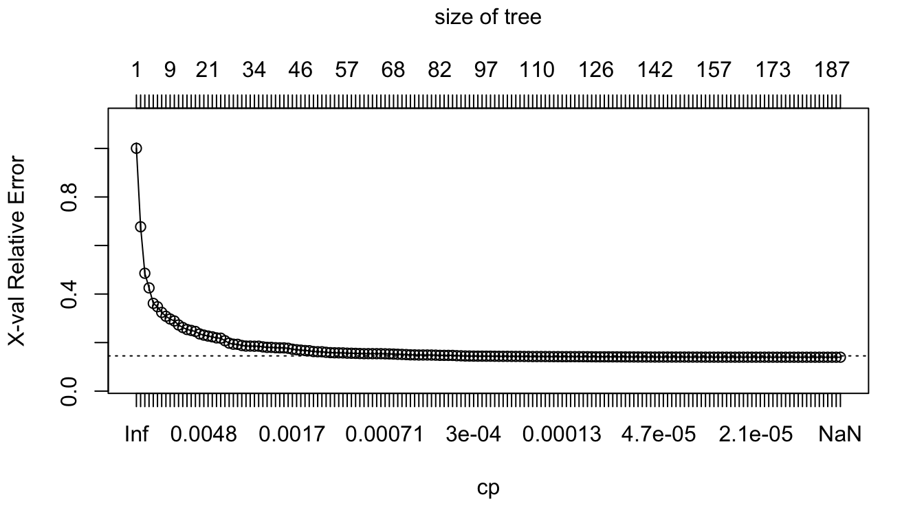

Figure 4.18: Relative error depending on the complexity parameter (10-fold cross-validation results), for the Seoul bike data.

The results of the cross-validation are stored in the cptable attribute of the result. The column CP (cost-complexity) corresponds to different values of $\lambda$, and the column xerror gives the resulting error.

head(large_tree$cptable)

##           CP nsplit rel error    xerror        xstd
## 1 0.33285801      0 1.0000000 1.0005565 0.021514547
## 2 0.19316259      1 0.6671420 0.6771662 0.015698709
## 3 0.07139607      2 0.4739794 0.4855051 0.012615119
## 4 0.05903069      3 0.4025833 0.4253927 0.010949168
## 5 0.01704578      4 0.3435527 0.3615918 0.009915513
## 6 0.01659517      5 0.3265069 0.3476690 0.009469073

Let us find the minimum value of the cost-parameter $\lambda$:

min_val <- 
  as_tibble(large_tree$cptable) %>%
  arrange(xerror) %>% 
  slice(1)

min_val

## # A tibble: 1 × 5
##           CP nsplit `rel error` xerror    xstd
##        <dbl>  <dbl>       <dbl>  <dbl>   <dbl>
## 1 0.00000162    185      0.0973  0.140 0.00544

Then, we can consider all the values of the cost-parameter within a 1-standard error deviation from that value:

candidates <- 
  as_tibble(large_tree$cptable) %>%
  filter( (xerror > min_val$xerror-min_val$xstd) & 
            (xerror < min_val$xerror+min_val$xstd)) %>% 
  arrange(desc(CP))
candidates

## # A tibble: 90 × 5
##          CP nsplit `rel error` xerror    xstd
##       <dbl>  <dbl>       <dbl>  <dbl>   <dbl>
##  1 0.000314     91       0.106  0.145 0.00546
##  2 0.000311     92       0.106  0.145 0.00546
##  3 0.000295     93       0.106  0.144 0.00546
##  4 0.000295     94       0.105  0.144 0.00546
##  5 0.000294     95       0.105  0.144 0.00546
##  6 0.000286     96       0.105  0.144 0.00546
##  7 0.000285     97       0.104  0.144 0.00546
##  8 0.000269     98       0.104  0.144 0.00546
##  9 0.000262     99       0.104  0.143 0.00546
## 10 0.000259    100       0.104  0.143 0.00545
## # … with 80 more rows

Among those candidates, we can pick up the values that results in the smallest subtree:

cp_val <- 
  candidates %>% 
  slice(1) %>% 
  magrittr::extract2("CP")
cp_val

## [1] 0.0003139774

Then, the tree can be pruned accordingly with this cost-complexity value, using the prune() function from {rpart}:

pruned_tree <- prune(large_tree, cp=cp_val)

Let us check the depth of the resulting tree:

nodes_pruned_tree <- as.numeric(rownames(pruned_tree$frame))
max(rpart:::tree.depth(nodes_pruned_tree))

## [1] 12

And for comparison, let us grow a smaller tree:

small_tree <- 
  rpart(rented_bike_count ~., 
        data = df_train %>% select(-y_binary, -date),
        method = "anova",
        maxdepth = 2,
        cp = 0,
        xval = 0)

# Number of nodes
nodes_small_tree <- as.numeric(rownames(small_tree$frame))
max(rpart:::tree.depth(nodes_small_tree))

## [1] 2

Let us compute the MSE on the test set:

pred_test_small <- predict(small_tree, newdata = df_test)
pred_test_large <- predict(large_tree, newdata = df_test)
pred_test_pruned <- predict(pruned_tree, newdata = df_test)

compute_mse <- function(observed, predicted){
  mean((observed-predicted)^2)
}

mse_small_tree <- 
  compute_mse(observed = df_test$rented_bike_count,
              predicted = pred_test_small)
mse_large_tree <- 
  compute_mse(observed = df_test$rented_bike_count,
              predicted = pred_test_large)
mse_pruned_tree <- 
  compute_mse(observed = df_test$rented_bike_count,
              predicted = pred_test_pruned)

mse <- scales::number(c(mse_small_tree, mse_large_tree,
                        mse_pruned_tree))
names(mse) <- c("Small", "Large", "Pruned")
mse

##     Small     Large    Pruned 
## "295 291" "164 097" "168 395"

Here, pruning the tree unfortunately produced a higher MSE in the test set. Let us have another look at pruning with our synthetic dataset this time.

Let us draw some new observations from the same data generating process.

set.seed(234)
x_new <- runif(n=n, min=0, max=10)
eps <- rnorm(n, 0, 4)
y_new <- f(x)+eps
df_sim_new <- tibble(x=x_new, y=y_new)
ggplot(mapping = aes(x = x, y = y)) +
  geom_line(data = tibble(x=seq(0, 10, by = .1), y=f(x)),
            colour = "black", size = 1.1, linetype = "dashed") +
  geom_point(data = df_sim %>% mutate(sample = "Train") %>% 
               bind_rows(
                 df_sim_new %>% mutate(sample = "Test")
               ),
             mapping = aes(colour = sample)) +
  scale_colour_manual("Sample", 
                      values = c("Train" = "#D55E00", "Test" = "#009E73"))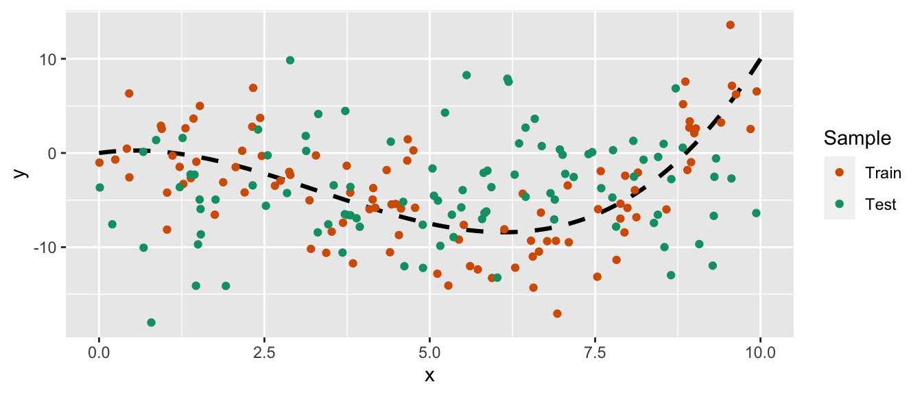

Figure 4.19: Synthetic data.

Let us build a large tree using the training sample:

part_tree_large <- 
  rpart(y ~ x, 
        data = df_sim,
        method = "anova",
        control = rpart.control(
          xval = 10, 
          cp = -1, 
          minbucket = 5)
  )
rpart.plot(part_tree_large)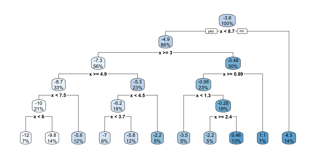

Figure 4.20: Unpruned tree.

The cost-parameter can be chosen thanks to the 10-fold cross-validation that was performed:

plotcp(part_tree_large)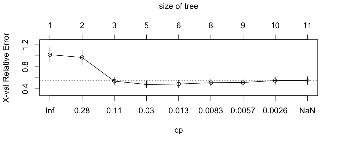

Figure 4.21: Relative error depending on the complexity parameter, for the synthetic data.

The same procedure to select $\lambda$ as that used on the Seoul bike data can be done. In a first step, we select the value that minimises the error:

min_val <- 
  as_tibble(part_tree_large$cptable) %>%
  arrange(xerror) %>% 
  slice(1)
min_val

## # A tibble: 1 × 5
##       CP nsplit `rel error` xerror   xstd
##    <dbl>  <dbl>       <dbl>  <dbl>  <dbl>
## 1 0.0185      4       0.344  0.479 0.0673

Then, we consider all values within a 1-standard error:

candidates <- 
  as_tibble(part_tree_large$cptable) %>%
  filter( (xerror > min_val$xerror-min_val$xstd) & 
            (xerror < min_val$xerror+min_val$xstd)) %>% 
  arrange(desc(CP))
candidates

## # A tibble: 5 × 5
##        CP nsplit `rel error` xerror   xstd
##     <dbl>  <dbl>       <dbl>  <dbl>  <dbl>
## 1 0.0482       2       0.440  0.539 0.0711
## 2 0.0185       4       0.344  0.479 0.0673
## 3 0.00927      5       0.325  0.486 0.0647
## 4 0.00749      7       0.307  0.511 0.0646
## 5 0.00429      8       0.299  0.514 0.0649

And finally, we pick the values among the candidates that produces the shallowest tree:

cp_val <- 
  candidates %>% 
  slice(1) %>% 
  magrittr::extract2("CP")
cp_val

## [1] 0.04824351

We can then prune the large tree:

pruned_tree <- prune(part_tree_large, cp=cp_val)
rpart.plot(pruned_tree)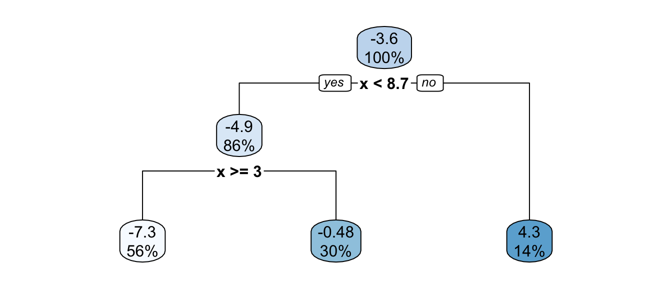

Figure 4.22: Pruned tree, synthetic data.

The depth of the pruned tree is indeed smaller:

nodes_pruned_tree <- as.numeric(rownames(pruned_tree$frame))
max(rpart:::tree.depth(nodes_pruned_tree))

## [1] 2

Let us visualise the boundaries of each tree:

boundaries <- 
  tibble(
    x = seq(0, 10, by = .1),
    y = predict(part_tree_large,
                newdata = tibble(x=seq(0, 10, by = .1)))
  )
boundaries_pruned <- 
  tibble(
    x = seq(0, 10, by = .1),
    y = predict(pruned_tree,
                newdata = tibble(x=seq(0, 10, by = .1)))
  )

ggplot(mapping = aes(x = x, y = y)) +
  geom_line(data = tibble(x=seq(0, 10, by = .1), y=f(x)),
            size = 1.1, linetype = "dashed", colour = "#AA2F2F") +
  geom_point(data = df_sim %>% mutate(sample = "Train") %>% 
               bind_rows(
                 df_sim_new %>% mutate(sample = "Test")
               ),
             mapping = aes(shape = sample)) +
  geom_step(data = boundaries %>% mutate(model = "Large Tree") %>% 
              bind_rows(
                boundaries_pruned %>% mutate(model = "Pruned Tree")
              ),
            mapping = aes(colour = model),
            # colour = "#005A8B",
            size = 1.5) +
  
  labs(title = str_c(
    "Decision boundaries for the **<span style='color:#E69F00'>",
    "large</span>** and for the **<span style='color:#56B4E9'>",
    "pruned</span>** trees")
  ) +
  scale_colour_manual("Boundary", 
                      values = c("Large Tree" = "#E69F00", 
                                 "Pruned Tree" = "#56B4E9")) +
  scale_shape_discrete("Dataset") +
  theme(
    plot.title = element_markdown(lineheight = 1.1),
    plot.title.position = "plot",
    legend.text = element_markdown(size = 11)
  )

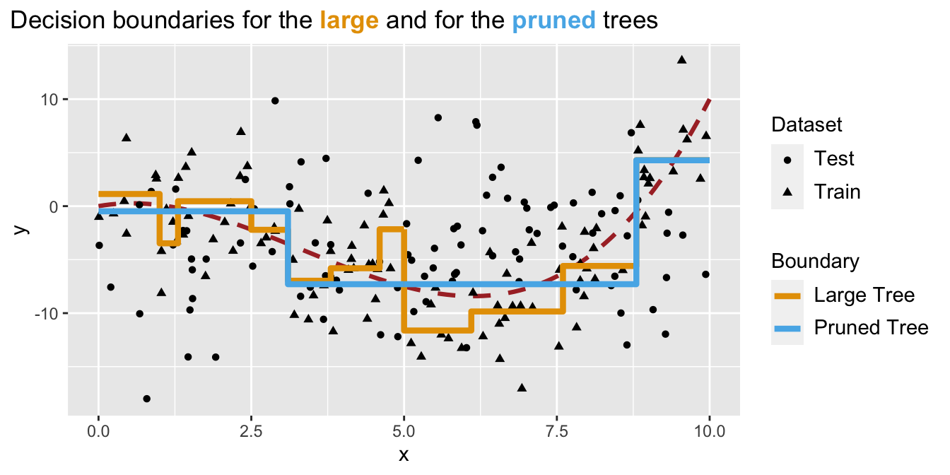
Figure 4.23: Decision boundaries are different after the tree was pruned.

Now, using these boundaries, let us compute the MSE on the unseen data (test set):

pred_test_large <- predict(part_tree_large, newdata = df_sim_new)
pred_test_pruned <- predict(pruned_tree, newdata = df_sim_new)

compute_mse <- function(observed, predicted){
  mean((observed-predicted)^2)
}


mse_large_tree <- 
  compute_mse(observed = df_sim_new$y, predicted = pred_test_large)
mse_pruned_tree <- 
  compute_mse(observed = df_sim_new$y, predicted = pred_test_pruned)

mse <- scales::number(c(mse_large_tree, mse_pruned_tree))
names(mse) <- c("Large", "Pruned")
print("MSE : \n")

## [1] "MSE : \n"

mse

##  Large Pruned 
##   "65"   "47"

We avoided overfitting by pruning the tree and ended-up with a lower MSE on the test.

4.3.3 Classification Trees

So far, we have considered a numerical target/response variable. Let us now consider the case where the predictor is categorical. This implies two changes:

the criterion used to select the variable/cutoff pairs can no longer be the RSS

we can use another metric, such as the classification error rate for example
or the Gini index, or the Entropy

the prediction made for each partition is no longer the average of the response variable

we can rely on a voting rule based on the proportions of the categories: for example, the proportions of each class can considered as the probabilities that the observations of a partition belong to each corresponding class.

Instead of using the classification error, it is more common to either use the Gini impurity index or the entropy to select the pair variable/cutoff that will be used to make a split.

The Gini impurity index at some node $\mathcal{N}$, as reminded in Emmanuel Flachaire’s course, is given by:

\[G(\mathcal{N}) = \sum_{k=1}^{K} p_k(1-p_k)= 1-\sum_{k=1}^{K} p_k^2,\]

where $p_k$ is the fraction of observations (or training samples) labeled with class $k$ in the node. If all the $p_k$ are close to 0, or to 1, the Gini impurity index has a small value: in such cases, there will be mostly observations from the same class, the node will be homogeneous. The Gini impurity index thus gives an idea of the total variance across the $K$ classes in a node.

Entropy is defined as follows: \[E(\mathcal{N}) = -\sum_{k=1}^K p_k \log(p_k)\] If the $p_k$ are all near 0 or near 1, the entropy will also be near 0.

After a split into two leaves $\mathcal{N}_{L}$ and $\mathcal{N}_{R}$, the Gini impurity index becomes:

\[G(\mathcal{N}_{L}, \mathcal{N}_{R}) = p_L G(\mathcal{N}_L) + p_R G(\mathcal{N}_R),\] where $p_L$ and $p_R$ are the proportion of observations in $\mathcal{N}_{L}$ and $\mathcal{N}_{R}$

In a similar fashion, the entropy becomes:

\[E(\mathcal{N}_{L}, \mathcal{N}_{R}) = p_L E(\mathcal{N}_L) + p_R E(\mathcal{N}_R).\]

Splits can be done as long as they substantially decrease impurity, i.e., when

\[\Delta = G(\mathcal{N}) - G(\mathcal{N}_L, \mathcal{N}_R) > \epsilon,\]

where $\epsilon$ is a threshold value set by the user.

The choice of the pair variable/cutoff can be done so as to select the one that minimises the impurity, i.e., the one that maximises $\Delta$.

Let us look at an example on the Seoul bike data. First, let us look at how some little changes need to be made when calling the rpart() function.

With regression trees, the argument method was set to "anova". Now that the variable of interest is categorical, we need to change the value to "class". By default, the Gini impurity index is used as the splitting index. If we want to use entropy, we can feed the argument parms with a list with the element split equal to "class".

Let us build a tree to predict our binary variable (recall that it is equal to "High" if the number of hourly bikes is greater than 300 and "Low" otherwise). Let us make sure that at least 20 observations are in a node before a split is attempted (minsplit = 20) and that there are at least 7 observations in each terminal leaves (minbucket = 7).

classif_tree_gini <- 
  rpart(y_binary ~., 
        data = df_train %>% select(-rented_bike_count, -date),
        method = "class",
        minsplit = 20,
        minbucket = 7,
        parms = list(split = "gini"))

The tree can be visualised thanks to the rpart.plot() function, as in the case of a regression tree. The argument extra allows to change the type of information reported on the graph. Here, since we have a binary response variable, the value is automatically set to 106 if not specified differently. It is made of two parts:

6: the probability of the second class only is reported
+100: the percentage of observations in the node is also added

rpart.plot(classif_tree_gini, extra = 106)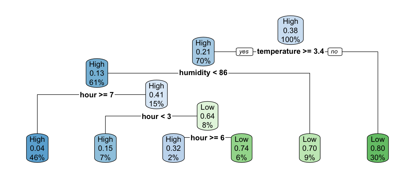

Figure 4.24: A first classification tree grown on Seoul bike data.

Here, at the top of the tree where 100% of observations are in the node, we read on the graph that the probability to be predicted as the second class (Low) is 0.38. This corresponds to the percentage of Low observations in the training dataset.

prop.table(table(df_train$y_binary))

## 
##      High       Low 
## 0.6151802 0.3848198

If the temperature is greater than or equal to 3.35 (we go to the left), we are left with 70% of the observations. In the resulting node, the probability to be classified as the second class (Low) is estimated at 0.21. This means that 21% of the observations in that node are labelled as Low:

df_train %>% 
  filter(temperature >= 3.35) %>%
  group_by(y_binary) %>% 
  count() %>% 
  ungroup() %>% 
  mutate(prop = round(n/sum(n), 2))

## # A tibble: 2 × 3
##   y_binary     n  prop
##   <chr>    <int> <dbl>
## 1 High      3754  0.79
## 2 Low        990  0.21

This concerns 70% of the observations:

df_train %>% 
  group_by(temperature < 3.35) %>% 
  count() %>% 
  ungroup() %>% 
  mutate(prop = n / sum(n))

## # A tibble: 2 × 3
##   `temperature < 3.35`     n  prop
##   <lgl>                <int> <dbl>
## 1 FALSE                 4744 0.701
## 2 TRUE                  2028 0.299

If the temperature is strictly lower than 3.35 (we go to the right), which concerns the remaining 30% of the observations, there are 20% of observations label with the first class (High) and 80%with the second (Low):

df_train %>% 
  filter(temperature < 3.35) %>%
  group_by(y_binary) %>% 
  count() %>% 
  ungroup() %>% 
  mutate(prop = round(n/sum(n), 2))

## # A tibble: 2 × 3
##   y_binary     n  prop
##   <chr>    <int> <dbl>
## 1 High       412   0.2
## 2 Low       1616   0.8

This is a terminal leaf node, so any observation that falls in it, the predicted class will be that of the most frequent class in that node. With this tree, if an observation has temperature >=3.35:

the probability that the number of bikes is of class “High” returned by the model will be 0.2
the probability that the number of bikes is of class “Low” returned by the model will be 0.8.

When calling the plot, we set extra=106. As $106 \mod 100 = 6$, only the probability of the second class is repord. Here is the list of available values that can be used (this list is extracted from the help page of the rpart() function):

1: the number of observations that fall in the node
2: the classification rate at the node (number of correct classifications and the number of observations in the node)
3: misclassification rate at the node (number of incorrect classifications and the number of observations in the node)
4: probability per class of observations in the node (conditioned on the node, sum across a node is 1)
5: like 4 but don’t display the fitted class
6: probability of the second class only. Useful for binary responses (the one we used)
7: like 6 but don’t display the fitted class
8: probability of the fitted class
9: probability relative to all observations – the sum of these probabilities across all leaves is 1. This is in contrast to the options above, which give the probability relative to observations falling in the node – the sum of the probabilities across the node is 1
10: like 9 but display the probability of the second class only. (Useful for binary responses).
11: like 10 but don’t display the fitted class

rpart.plot(classif_tree_gini, extra = 102)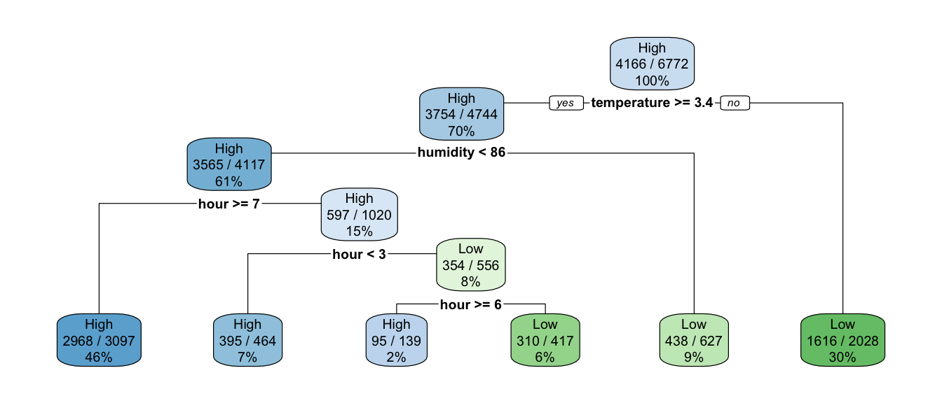

Figure 4.25: Showing the classification rate at the node.

If we want to use entropy instead of the Gini impurity index as the splitting index, all we need to do is to change the value of the element split in the list given to the parms argument so that it becomes "information" instead of "gini".

classif_tree_entropy <- 
  rpart(y_binary ~., 
        data = df_train %>% select(-rented_bike_count, -date),
        method = "class",
        parms = list(split = "information"))
rpart.plot(classif_tree_entropy)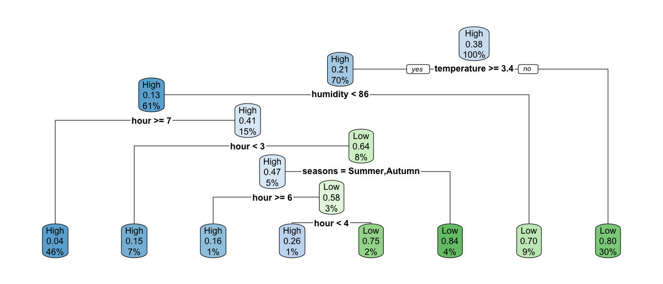

Figure 4.26: Classification tree build using entropy instead of gini to measure impurity index.

Similarly to what we did with regression trees, let us have a closer look at how the splitting rule is performed. Let us consider temperature as the splitting variable, and let us set a cutoff value of 10.

variable_split <- "temperature"
threshold <- 10

Let us consider the root as the current node:

current_node <- df_train

The proportion of each class, $p_k$, can be computed as follows:

prop_current_node <- 
  current_node %>% 
  group_by(y_binary) %>% 
  count() %>% 
  ungroup() %>% 
  mutate(p_k = n / sum(n))
prop_current_node

## # A tibble: 2 × 3
##   y_binary     n   p_k
##   <chr>    <int> <dbl>
## 1 High      4166 0.615
## 2 Low       2606 0.385

The Gini impurity index in that current node is:

gini_node <- 
  prop_current_node %>% 
  mutate(g_k = p_k*(1-p_k)) %>% 
  magrittr::extract2("g_k") %>% 
  sum()
gini_node

## [1] 0.4734671

Let us define a function that computes the Gini impurity index on a given node:

#' @param data_node tibble/data.frame with the data of the node
#' @param target name of the target variable (discrete variable)
compute_gini <- function(data_node, target){
  
  prop_current_node <- 
    data_node %>% 
    group_by(!!sym(target)) %>% 
    count() %>% 
    ungroup() %>% 
    mutate(p_k = n / sum(n))
  
  prop_current_node %>% 
    mutate(g_k = p_k*(1-p_k)) %>% 
    magrittr::extract2("g_k") %>% 
    sum()
}

Which can be used this way:

compute_gini(current_node, "y_binary")

## [1] 0.4734671

Let us split the data into two partitions, depending on the splitting variable and the tested cutoff:

left_node <- 
  current_node %>% 
  filter(temperature < threshold)

right_node <- 
  current_node %>% 
  filter(temperature >= threshold)

The proportions of observations in each node $p_L$ and $p_R$ can be computed as follows:

p_L <- nrow(left_node) / nrow(current_node)
p_R <- nrow(right_node) / nrow(current_node)
cat(str_c("Prop left: ", p_L, "\n", "Prop right: ", p_R))

## Prop left: 0.427495569994093
## Prop right: 0.572504430005907

The Gini impurity coefficient in left and right nodes:

gini_left <- compute_gini(left_node, "y_binary")
gini_right <- compute_gini(right_node, "y_binary")

c(gini_left, gini_right)

## [1] 0.4353491 0.2749603

The weighted average of the Gini impurity indices:

gini_l_r <- p_L*gini_left + p_R * gini_right
gini_l_r

## [1] 0.3435258

Let us recap:

the Gini impurity index in the current node is equal to 0.4734671
the Gini impurity index after the split is equal to 0.3435258

Hence, the decrease in impurity ($\Delta$) after the split is equal to:

gini_node - gini_l_r

## [1] 0.1299412

Equivalently, the split allowed to reduce the impurity by -0.27%:

(gini_l_r - gini_node)/gini_node

## [1] -0.2744462

Let us wrap-up the previous code in a function:

gini_split <- function(data_node, variable_to_predict, 
                       variable_split, threshold,
                       minbucket){
  
  if(is.numeric(data_node[[variable_split]])){
    left_node <- 
      data_node %>% 
      filter(!!sym(variable_split) < threshold)
    
    right_node <- 
      data_node %>% 
      filter(!!sym(variable_split) >= threshold)
  }else{
    left_node <- 
      data_node %>% 
      filter(!!sym(variable_split) %in% threshold)
    
    right_node <- 
      data_node %>% 
      filter( !( !!sym(variable_split) %in% threshold ))
  }
  
  # If there is less than a given number of obs in the leaves
  # warning
  warning_min_bucket <- 
    any( table(left_node[[variable_to_predict]]) < minbucket) |
    any( table(right_node[[variable_to_predict]]) < minbucket)
  
  # Proportions of obs in the resulting leaves
  p_L <- nrow(left_node) / nrow(current_node)
  p_R <- nrow(right_node) / nrow(current_node)
  
  # Gini in leaves
  gini_left <- compute_gini(left_node, "y_binary")
  gini_right <- compute_gini(right_node, "y_binary")
  
  gini_l_r <- p_L*gini_left + p_R * gini_right
  
  list(gini_l_r = gini_l_r, warning_min_bucket = warning_min_bucket)
}

This function can then be applied as follows:

gini_split(
  data_node = df_train, variable_to_predict = "y_binary",
  variable_split = "temperature", threshold = 10, minbucket = 7)

## $gini_l_r
## [1] 0.3435258
## 
## $warning_min_bucket
## [1] FALSE

Let us consider multiple cutoffs:

number_of_cuts <- 1000
thresholds <- 
  seq(min(df_train$temperature), max(df_train$temperature),
      length.out = number_of_cuts)

We can loop over these values of cutoff.

gini_leaves <- 
  map(thresholds, ~gini_split(
    data_node = df_train, variable_to_predict = "y_binary",
    variable_split = "temperature", threshold = ., minbucket = 7))

The resulting values of $G(\mathcal{N}_L, \mathcal{N}_R)$ can be stored in a table:

gini_leaves_df <- 
  tibble(
    g_leaves = map_dbl(gini_leaves, "gini_l_r"),
    warning_min_bucket = map_lgl(gini_leaves, "warning_min_bucket"),
    threshold = thresholds) %>% 
  mutate(delta = gini_node - g_leaves,
         warning_min_bucket = factor(
           warning_min_bucket, levels = c(TRUE, FALSE),
           labels = c("Not permitted", "Permitted")))
gini_leaves_df

## # A tibble: 1,000 × 4
##    g_leaves warning_min_bucket threshold     delta
##       <dbl> <fct>                  <dbl>     <dbl>
##  1    0.473 Permitted              -17.8 0        
##  2    0.473 Not permitted          -17.7 0.0000437
##  3    0.473 Not permitted          -17.7 0.0000437
##  4    0.473 Not permitted          -17.6 0.0000437
##  5    0.473 Not permitted          -17.6 0.0000437
##  6    0.473 Not permitted          -17.5 0.0000437
##  7    0.473 Not permitted          -17.5 0.0000704
##  8    0.473 Not permitted          -17.4 0.000158 
##  9    0.473 Not permitted          -17.3 0.000158 
## 10    0.473 Not permitted          -17.3 0.000158 
## # … with 990 more rows

When the threshold lead to a split in which there were too few observations (less than 7) in a leaf, we labelled the result as “Not permitted” in the warming_min_bucket column. The improvement obtained with each tested cutoff value can be visualised on a graph:

ggplot(data = gini_leaves_df, 
       mapping = aes(x = threshold, y = delta)) +
  geom_point(mapping = aes(colour = warning_min_bucket)) +
  scale_colour_manual(
    "Threshold", 
    values = c("Permitted" = "blue", "Not permitted" = "red")) +
  labs(x = "Temperature threshold") +
  theme(plot.title.position = "plot")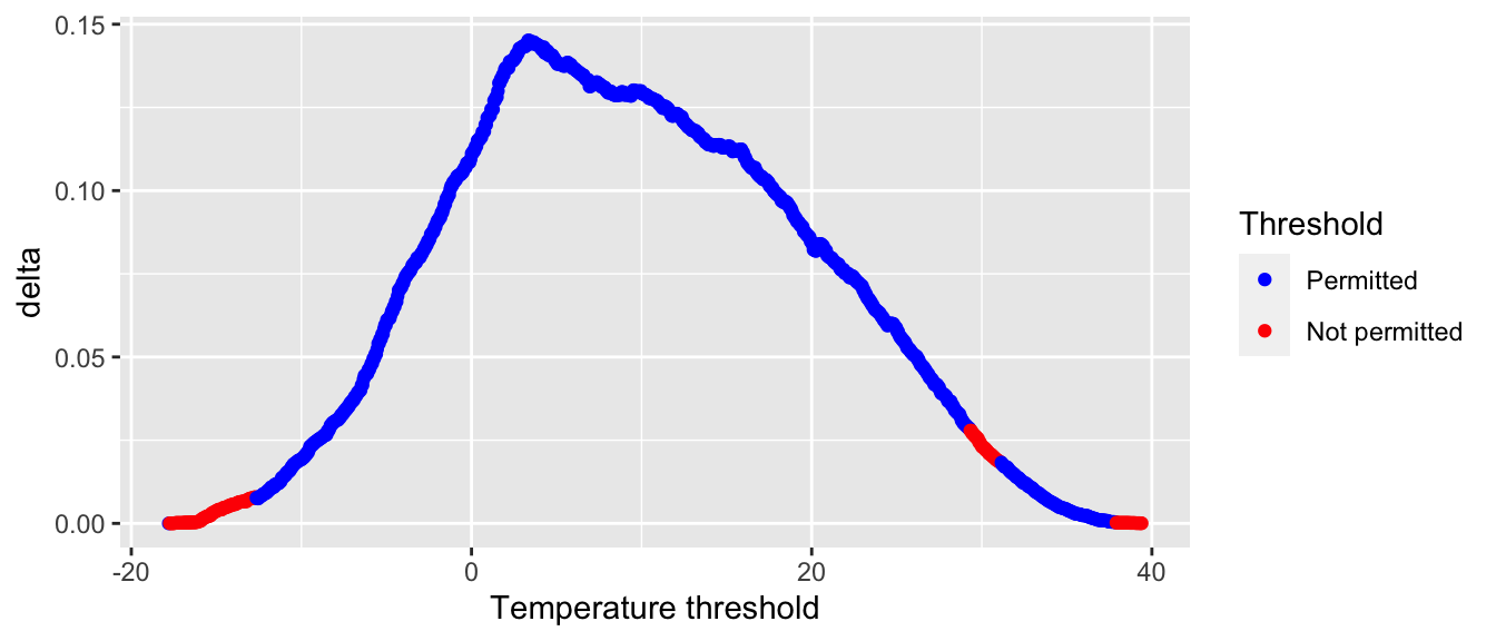

Figure 4.27: Decrease in the impurity design.

gini_leaves_df %>% 
  filter(warning_min_bucket == "Permitted") %>% 
  arrange(desc(delta))

## # A tibble: 852 × 4
##    g_leaves warning_min_bucket threshold delta
##       <dbl> <fct>                  <dbl> <dbl>
##  1    0.328 Permitted               3.33 0.145
##  2    0.328 Permitted               3.39 0.145
##  3    0.329 Permitted               3.44 0.145
##  4    0.329 Permitted               3.50 0.145
##  5    0.329 Permitted               3.61 0.145
##  6    0.329 Permitted               3.67 0.145
##  7    0.329 Permitted               3.73 0.144
##  8    0.329 Permitted               3.79 0.144
##  9    0.329 Permitted               3.56 0.144
## 10    0.330 Permitted               3.84 0.144
## # … with 842 more rows

The best threshold for the split made with temperature is the one, among the permitted solutions, that leads to the highest impurity decrease:

gini_l_r_temperature <- 
  gini_leaves_df %>% 
  filter(warning_min_bucket == "Permitted") %>% 
  arrange(desc(delta))
gini_l_r_temperature

## # A tibble: 852 × 4
##    g_leaves warning_min_bucket threshold delta
##       <dbl> <fct>                  <dbl> <dbl>
##  1    0.328 Permitted               3.33 0.145
##  2    0.328 Permitted               3.39 0.145
##  3    0.329 Permitted               3.44 0.145
##  4    0.329 Permitted               3.50 0.145
##  5    0.329 Permitted               3.61 0.145
##  6    0.329 Permitted               3.67 0.145
##  7    0.329 Permitted               3.73 0.144
##  8    0.329 Permitted               3.79 0.144
##  9    0.329 Permitted               3.56 0.144
## 10    0.330 Permitted               3.84 0.144
## # … with 842 more rows

We obtain a value very close to that reported in the graph (the specific 3.35 value was not tested in our sequence of cutoffs).

To be exhaustive, we should consider all other variables, and not only temperature, to select the best pair of variable/cutoff to perform the split.

If we look at the value reported in the improve column of the splits element returned by the rpart() function, we actually get $n_\mathcal{I} \times \Delta$, where $n_\mathcal{I}$ is the number of observations in the current node.

head(classif_tree_gini$splits)

##                       count ncat     improve index       adj
## temperature            6772    1 982.9149704  3.35 0.0000000
## seasons                6772    4 793.1418098  1.00 0.0000000
## month                  6772   12 793.1418098  2.00 0.0000000
## dew_point_temperature  6772    1 539.9467740  2.65 0.0000000
## hour                   6772    1 434.9381343  6.50 0.0000000
## seasons                   0    4   0.9208506  3.00 0.7357002

Compared with:

nrow(current_node) * (gini_node-gini_l_r_temperature$g_leaves[1])

## [1] 982.915

More explanations on the rows of that table will be provided afterwards in this section and in the variable importance section.

Let us just give a few examples of other competitor variables. The element splits returned by the rpart() function contains, among other things, some information relative to those competitor variables. In our example, the first five rows of this split table report the improvement in the fit depending on the variable used to make the split (the value reported concerns the best cutoff for each variable tested).

head(classif_tree_gini$splits, 5)

##                       count ncat  improve index adj
## temperature            6772    1 982.9150  3.35   0
## seasons                6772    4 793.1418  1.00   0
## month                  6772   12 793.1418  2.00   0
## dew_point_temperature  6772    1 539.9468  2.65   0
## hour                   6772    1 434.9381  6.50   0

Let us recall that the value in the improve column correspond to $n_\mathcal{I} \times \Delta$. The Gini impurity index in the root node is:

(gini_initial <- compute_gini(df_train, "y_binary"))

## [1] 0.4734671

If we use the temperature variable as the splitting one, the increase in the goodness of fit (as measured by the average of the Gini impurity index computed on the two resulting leaves) can be obtained with the following code:

gini_split_temperature <- 
  gini_split(
    data_node = df_train, variable_to_predict = "y_binary",
    variable_split = "temperature", threshold = 3.35, minbucket = 7)

nrow(df_train) * (gini_initial - gini_split_temperature$gini_l_r)

## [1] 982.915

For the variable seasons:

gini_split_seasons <- 
  gini_split(
    data_node = df_train, variable_to_predict = "y_binary",
    variable_split = "seasons", threshold = c("Winter"), minbucket = 7)

nrow(df_train) * (gini_initial - gini_split_seasons$gini_l_r)

## [1] 793.1418

For the variable month:

gini_split_month <- 
  gini_split(
    data_node = df_train, variable_to_predict = "y_binary",
    variable_split = "month", threshold = c("Jan","Feb","Dec"), minbucket = 7)

nrow(df_train) * (gini_initial - gini_split_month$gini_l_r)

## [1] 793.1418

and so on.

4.3.4 Variable Importance

For a given node, the variable that is eventually used to perform the split is called a primary variable. We have seen that the choice of the primary split is done using a metric that computes the goodness of fit (for example, the Gini Index or the Impurity index in the case of a classification tree).

To compute the importance of a variable, we can also consider the surrogate variables. These variables are used to try to handle missing values. Once a primary split has been obtained, another variable can be used to try to obtain a similar assignment in the left and right nodes. If there are missing values when we use the primary split, then a surrogate split can be used to make the prediction. The surrogate variable may thus be relatively important if they are able to reproduce more or less the same results as the split obtained with the primary variable.

Let us have a quick look at how to measure the capacity of a surrogate variable to reproduce the same results as that obtained with a primary variable. To do so, we depart from what is explained in Section 3.4 of the vignette of {rpart}.

Once again, let us focus on the root node.

current_node <- df_train

The primary variable for that split, is temperature, and the best cutoff is 3.35. Let us use the variable seasons as a surrogate. Among all the possible combinations of splitting rules for seasons, the one that gives the best results in terms of error rate is "Winter".

tmp <- 
  current_node %>% 
  mutate(
    # Primary split
    leave_primary = case_when(
      temperature < 3.35 ~ "left prim.",
      temperature >= 3.35 ~ "right prim."),
    # Surrogate split
    leave_surrogate = case_when(
      seasons == "Winter" ~ "left surr.",
      seasons != "Winter" ~ "right surr."
    ))

Let us look at the results:

confusion <- table(tmp$leave_primary, tmp$leave_surrogate, exclude = NULL)
confusion

##              
##               left surr. right surr.
##   left prim.        1826         202
##   right prim.        334        4410

Using the surrogate, 1826 + 4410 = 6236 out of the 6772 observations are sent to the correct direction. This corresponds to an average proportion of correctly sent observations of 0.9208506.

correct_direction <- (confusion["left prim.", "left surr."] + confusion["right prim.", "right surr."])
correct_direction

## [1] 6236

# Proportion
correct_direction/sum(confusion)

## [1] 0.9208506

The majority rule gets 4744 correct:

maj_rule_correct <- sum(confusion["right prim.", ])
maj_rule_correct

## [1] 4744

Hence, the adjusted agreement is:

adjust <- (correct_direction - maj_rule_correct) / (sum(confusion) - maj_rule_correct)
adjust

## [1] 0.7357002

The relative importance of a variable is computed by accounting for when it appears as a primary variable, and also when it appears as a surrogate variable.

The composite metrics can be accessed through the variable.importance element of the result returned by the rpart() function.

classif_tree_gini$variable.importance

##           temperature                 month               seasons 
##             989.14552             723.13074             723.13074 
## dew_point_temperature                  hour              humidity 
##             681.60244             372.01312             371.05659 
##                  year              snowfall              rainfall 
##             244.27473             179.32867             148.96535 
##       solar_radiation            visibility            wind_speed 
##              88.03473              51.16607              34.21947

When we call the summary() function on the result of the rpart() function, we get rounded values of the relative importance of the variables:

round(100 * classif_tree_gini$variable.importance / 
        sum(classif_tree_gini$variable.importance))

##           temperature                 month               seasons 
##                    21                    16                    16 
## dew_point_temperature                  hour              humidity 
##                    15                     8                     8 
##                  year              snowfall              rainfall 
##                     5                     4                     3 
##       solar_radiation            visibility            wind_speed 
##                     2                     1                     1

The only thing that remains is to understand how those values are obtained. To that end, we need to better understand the content of the split element that is returned by the rpart() function. In this table, primary variables, competitor variables (variables that would have produce a relatively close result in term of increase in the goodness of fit), and surrogate variables are given in a jumble.

splits_df <- 
  as_tibble(classif_tree_gini$splits, rownames = "variable")
splits_df

## # A tibble: 43 × 6
##    variable              count  ncat improve   index   adj
##    <chr>                 <dbl> <dbl>   <dbl>   <dbl> <dbl>
##  1 temperature            6772     1 983.       3.35 0    
##  2 seasons                6772     4 793.       1    0    
##  3 month                  6772    12 793.       2    0    
##  4 dew_point_temperature  6772     1 540.       2.65 0    
##  5 hour                   6772     1 435.       6.5  0    
##  6 seasons                   0     4   0.921    3    0.736
##  7 month                     0    12   0.921    4    0.736
##  8 dew_point_temperature     0     1   0.907   -3.85 0.688
##  9 year                      0     1   0.775 2018.   0.249
## 10 snowfall                  0    -1   0.755    0.05 0.182
## # … with 33 more rows

We can use the results of table contained in the element frame of the result returned by the rpart() function. More specifically, the columns ncompete and nsurrogate tell us how many competitor variables and how many surrogate variables are reported in the table in the splits element, just after the primary variable.

head(classif_tree_gini$frame)

##            var    n   wt  dev yval  complexity ncompete nsurrogate     yval2.V1
## 1  temperature 6772 6772 2606    1 0.462010744        4          5 1.000000e+00
## 2     humidity 4744 4744  990    1 0.095548734        4          3 1.000000e+00
## 4         hour 4117 4117  552    1 0.029163469        4          4 1.000000e+00
## 8       <leaf> 3097 3097  129    1 0.000000000        0          0 1.000000e+00
## 9         hour 1020 1020  423    1 0.029163469        4          5 1.000000e+00
##        yval2.V2     yval2.V3     yval2.V4     yval2.V5 yval2.nodeprob
## 1  4.166000e+03 2.606000e+03 6.151802e-01 3.848198e-01   1.000000e+00
## 2  3.754000e+03 9.900000e+02 7.913153e-01 2.086847e-01   7.005316e-01
## 4  3.565000e+03 5.520000e+02 8.659218e-01 1.340782e-01   6.079445e-01
## 8  2.968000e+03 1.290000e+02 9.583468e-01 4.165321e-02   4.573243e-01
## 9  5.970000e+02 4.230000e+02 5.852941e-01 4.147059e-01   1.506202e-01
##  [ getOption("max.print") est atteint -- ligne 1 omise ]

We can thus create a vector that can be added to the table that contains the information on the splits.

# Position of the primary variables in `frame`
ind_primary <- which(classif_tree_gini$frame$var != "<leaf>")

type_var_df <- 
  classif_tree_gini$frame %>% 
  slice(ind_primary) %>% 
  select(ncompete, nsurrogate)

type_var <- NULL
for(i in 1:nrow(type_var_df)){
  type_var <- c(type_var, "primary", 
                rep("competitor", type_var_df[i, "ncompete"]),
                rep("surrogate", type_var_df[i, "nsurrogate"])
  ) 
}
type_var

##  [1] "primary"    "competitor" "competitor" "competitor" "competitor"
##  [6] "surrogate"  "surrogate"  "surrogate"  "surrogate"  "surrogate" 
## [11] "primary"    "competitor" "competitor" "competitor" "competitor"
## [16] "surrogate"  "surrogate"  "surrogate"  "primary"    "competitor"
## [21] "competitor" "competitor" "competitor" "surrogate"  "surrogate" 
## [26] "surrogate"  "surrogate"  "primary"    "competitor" "competitor"
## [31] "competitor" "competitor" "surrogate"  "surrogate"  "surrogate" 
## [36] "surrogate"  "surrogate"  "primary"    "competitor" "competitor"
## [41] "competitor" "competitor" "surrogate"

This vector can then be added in splits_df:

splits_df <- splits_df %>% mutate(type_var = type_var)
splits_df

## # A tibble: 43 × 7
##    variable              count  ncat improve   index   adj type_var  
##    <chr>                 <dbl> <dbl>   <dbl>   <dbl> <dbl> <chr>     
##  1 temperature            6772     1 983.       3.35 0     primary   
##  2 seasons                6772     4 793.       1    0     competitor
##  3 month                  6772    12 793.       2    0     competitor
##  4 dew_point_temperature  6772     1 540.       2.65 0     competitor
##  5 hour                   6772     1 435.       6.5  0     competitor
##  6 seasons                   0     4   0.921    3    0.736 surrogate 
##  7 month                     0    12   0.921    4    0.736 surrogate 
##  8 dew_point_temperature     0     1   0.907   -3.85 0.688 surrogate 
##  9 year                      0     1   0.775 2018.   0.249 surrogate 
## 10 snowfall                  0    -1   0.755    0.05 0.182 surrogate 
## # … with 33 more rows

Let us focus once again on the variable temperature.

variable_of_interest <- "temperature"

Each primary split for this variable is credited with the improvement value:

var_imp <- 
  splits_df %>% 
  filter(variable == variable_of_interest, type_var == "primary") %>% 
  magrittr::extract2("improve") %>% 
  sum()
var_imp

## [1] 982.915

And each surrogate split where temperature is used gets split$adj times the primary split’s value. We thus need to add a column that gives the primary split’s value for each surrogate variable.

splits_df <- 
  splits_df %>% 
  mutate(primary_split_value = 
           ifelse(type_var == "primary", improve, NA)) %>% 
  fill(primary_split_value) %>% 
  mutate(primary_split_value = 
           ifelse(type_var != "surrogate", NA, primary_split_value))
splits_df

## # A tibble: 43 × 8
##    variable        count  ncat improve   index   adj type_var  primary_split_va…
##    <chr>           <dbl> <dbl>   <dbl>   <dbl> <dbl> <chr>                 <dbl>
##  1 temperature      6772     1 983.       3.35 0     primary                 NA 
##  2 seasons          6772     4 793.       1    0     competit…               NA 
##  3 month            6772    12 793.       2    0     competit…               NA 
##  4 dew_point_temp…  6772     1 540.       2.65 0     competit…               NA 
##  5 hour             6772     1 435.       6.5  0     competit…               NA 
##  6 seasons             0     4   0.921    3    0.736 surrogate              983.
##  7 month               0    12   0.921    4    0.736 surrogate              983.
##  8 dew_point_temp…     0     1   0.907   -3.85 0.688 surrogate              983.
##  9 year                0     1   0.775 2018.   0.249 surrogate              983.
## 10 snowfall            0    -1   0.755    0.05 0.182 surrogate              983.
## # … with 33 more rows

We can compute the contribution of the variable temperature each time it is a surrogate variable to the importance metric:

var_imp_surrogate <- 
  splits_df %>% 
  filter(variable == variable_of_interest,
         type_var == "surrogate") %>%
  mutate(imp_contrib = primary_split_value*adj) %>% 
  magrittr::extract2("imp_contrib") %>% 
  sum()
var_imp_surrogate

## [1] 6.230553

When adding the two parts, we obtain the importance measure of the temperature variable:

var_imp+var_imp_surrogate

## [1] 989.1455

To compute the importance of all variables at once:

splits_df %>% 
  mutate(importance = ifelse(type_var == "primary", improve, 0),
         importance = ifelse(
           type_var == "surrogate", 
           importance+primary_split_value*adj, importance)) %>% 
  group_by(variable) %>% 
  summarise(importance = sum(importance)) %>% 
  arrange(desc(importance))

## # A tibble: 12 × 2
##    variable              importance
##    <chr>                      <dbl>
##  1 temperature                989. 
##  2 month                      723. 
##  3 seasons                    723. 
##  4 dew_point_temperature      682. 
##  5 hour                       372. 
##  6 humidity                   371. 
##  7 year                       244. 
##  8 snowfall                   179. 
##  9 rainfall                   149. 
## 10 solar_radiation             88.0
## 11 visibility                  51.2
## 12 wind_speed                  34.2

We get the same values as those reported in the result of rpart() (although the values are rounded in the tibble):

classif_tree_gini$variable.importance

##           temperature                 month               seasons 
##             989.14552             723.13074             723.13074 
## dew_point_temperature                  hour              humidity 
##             681.60244             372.01312             371.05659 
##                  year              snowfall              rainfall 
##             244.27473             179.32867             148.96535 
##       solar_radiation            visibility            wind_speed 
##              88.03473              51.16607              34.21947

We can plot those values using a barplot:

as_tibble(classif_tree_gini$variable.importance,
          rownames = "variable") %>% 
  mutate(rel_importace = 100*value / sum(value)) %>% 
  ggplot(data = ., 
         mapping = aes(x = rel_importace, 
                       y = fct_reorder(variable, rel_importace))) +
  geom_bar(stat = "identity") +
  labs(x = "relative importance", y = NULL) +
  theme(plot.title.position = "plot")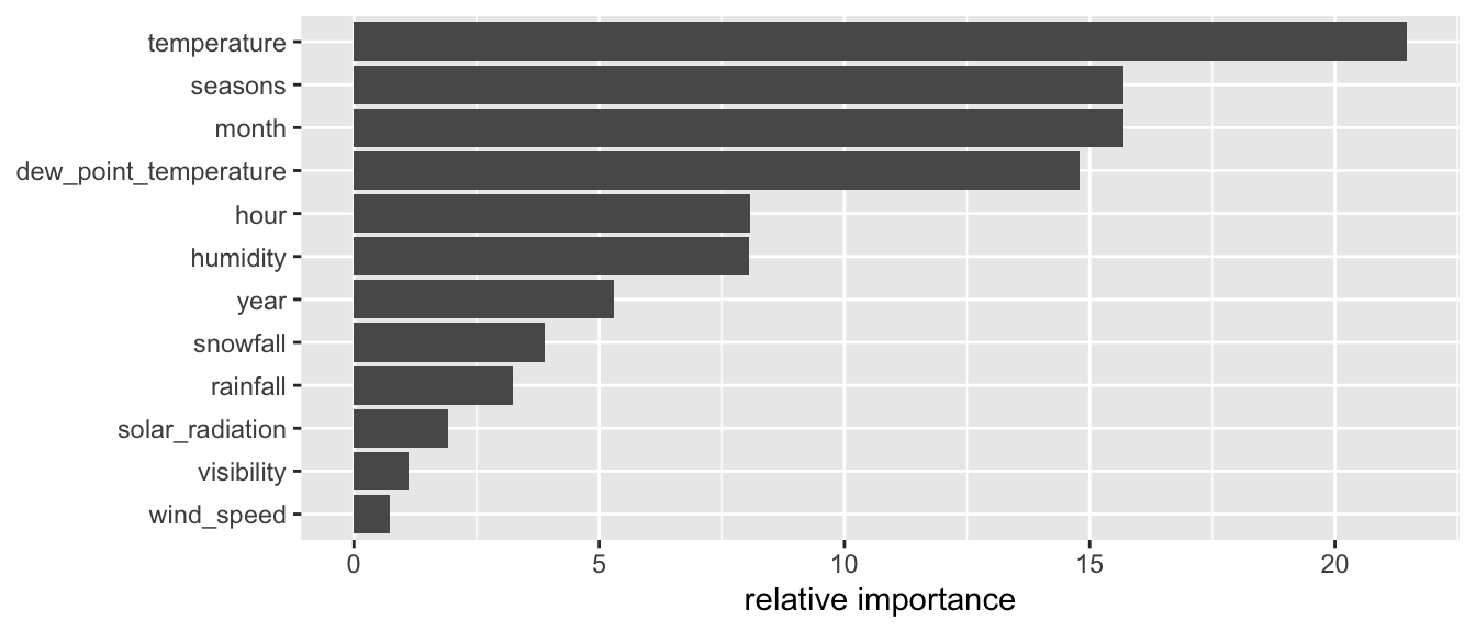

Figure 4.28: Variable importance for the Classification Tree.

4.4 Ensemble Methods

As explained in James et al. (2021), the predictive performances of trees are not very competitive with other machine learning algorithm. In addition, small changes in the data can lead to large changes in the final estimated tree. A way to overcome these issues is to rely on aggregating multiple decision trees. The basic idea is to build weak learners, i.e., simple models that will provide predictions that may be mediocre but are consistently better than an random guessing. These weak learners can then be combined together: this forms an ensemble method.

This section will present three methods: bagging, random forest, and then boosting. Each of these methods are build using regression trees or classification trees as weak learners.

4.4.1 Bagging

Bagging (bootstrap aggregating) consists in generating multiple bootstrap from the data, estimate a tree model on each sample (building weak learners), and then averaging the predictions made by the weak learners to form new predictions. They were introduced in Leo Breiman (1996).

The new predictions are made as follows:

in the case of a regression problem, the average of the values predicted by the weak learners can be calculated.
in the case of a classification problem, a majority vote can be used or the estimated probabilities for each class can be averaged.

Proceeding this way offers the advantage to reduce the variance of the model. A known issue with regression trees is that they are sensitive so small changes in the data and therefore suffer from high variance. If another variable is used to make a split, or if a cutoff is changed, the output can be greatly modified. This issue can be reduced thanks to bootstrapping. Aggregating the results will lower the variance. From this, we understand that if we want the bootstrapping and aggregation to be efficient in lowering the variance, the weak learners need to be high variance models (otherwise, they would yield approximately the same results regardless of the changes made, and taking the average of values which do not vary much would not greatly diminish the variance).

If we want to get an unbiased prediction, with low variance, it may be a good idea to use weak learners with low bias. We can therefore use deep trees. Even if those deep trees will suffer from high variance, the bagging procedure will lower this variance.

A disadvantage of bagging compared to a regression or classification tree is that the results are no longer interpretable using a decision tree.

Let us illustrate how the method works with a regression problem. We use the same synthetic data that was used with the regression trees.

set.seed(123)
n <- 100
x <- runif(n=n, min=0, max=10)
eps <- rnorm(n, 0, 4)
f <- function(x) .1*x^3-1*x^2+x
y <- f(x)+eps
df_sim <- tibble(x=x, y=y)

We will create $B=100$ bootstrap resamples of the data. On each sample, we will build an unpruned regression tree (cp=0).

n <- nrow(df_sim)
nb_bagg <- 100
baggin_models <- vector(mode = "list", length = nb_bagg)
for(i in 1:nb_bagg){
  
  ind_x <- sample(1:n, size = n, replace = TRUE)
  df_tmp <- df_sim %>% slice(ind_x)
  
  cart <- 
    rpart(y ~ x, 
          data = df_tmp,
          method = "anova",
          control = rpart.control(cp = 0)
    )
  
  baggin_models[[i]] <- cart
  
}

Each element of the object baggin_models contains a weak learner:

baggin_models[[1]]

## n= 100 
## 
## node), split, n, deviance, yval
##       * denotes terminal node
## 
##  1) root 100 3845.46700  -4.0083810  
##    2) x< 8.465409 89 2476.34100  -5.2637170  
##      4) x>=3.036704 60  940.14170  -7.6988470  
##        8) x< 7.538915 44  752.24400  -8.4066460  
##         16) x>=5.029507 24  291.07670  -9.9336230  
##           32) x< 6.665854 14  108.26800 -10.7958400 *
##           33) x>=6.665854 10  157.82980  -8.7265200 *
##         17) x< 5.029507 20  338.05560  -6.5742730  
##           34) x< 3.99258 10  107.92920  -9.0906140 *
##           35) x>=3.99258 10  103.48700  -4.0579310 *
##        9) x>=7.538915 16  105.23620  -5.7524020 *
##      5) x< 3.036704 29  444.28740  -0.2255172  
##       10) x>=1.637487 12   77.95662  -1.9062080 *
##       11) x< 1.637487 17  308.50700   0.9608528 *
##    3) x>=8.465409 11   94.10378   6.1484350 *

Let us create a function that will make predictions on each weak learner on some data. The predictions for a given point obtained with the weak learners will then be averaged.

predict_bagged <- function(baggin_models, newdata){
  map(baggin_models, ~predict(., newdata = newdata)) %>% 
    bind_cols(
      .name_repair = ~ vctrs::vec_as_names(
        ..., repair = "unique", quiet = TRUE)) %>% 
    rowMeans()
}

For simplicity, let us create some new data ranging from 0 to 10:

new_data <- tibble(x = seq(0, 10, by = .1))

The predictions can then easily be calculated:

pred_bagging <- predict_bagged(baggin_models, new_data)
head(pred_bagging)

## [1] -0.1701479 -0.1701479 -0.1701479 -0.1701479 -0.1701479 -0.2358646

Let us plot the observed values and the predictions obtained with bagging:

df_plot <- 
  new_data %>% 
  mutate(pred = pred_bagging,
         expected = f(x))

ggplot(mapping = aes(x = x, y = y)) +
  geom_point(data = df_sim) +
  geom_line(data = df_plot %>% pivot_longer(-x, values_to = "y"), 
            mapping = aes(colour = name),
            size = 1.1)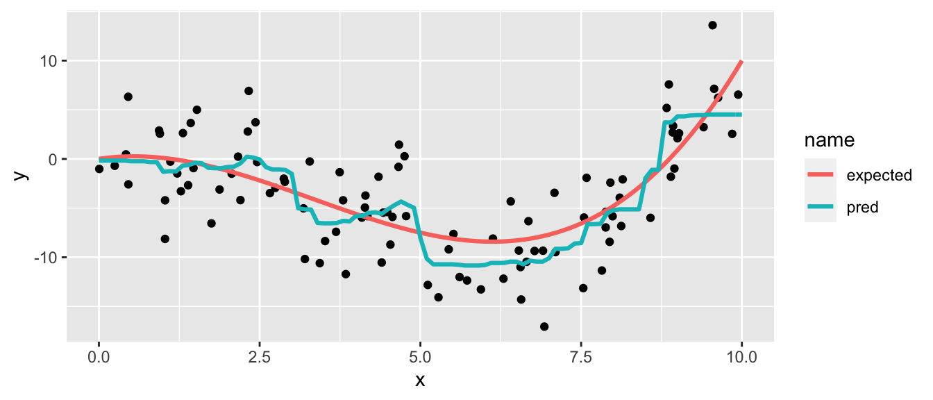

Figure 4.29: Bagging with 100 bootstrap training sets.

4.4.1.1 Number of Trees

What happens when more trees are grown? To have an idea, let us make the number of trees vary. A little function that samples from the data and then grow an unpruned tree may help.

train_weak_learner <- function(data, formula, method, control){
  n <- nrow(data)
  ind_x <- sample(1:n, size = n, replace = TRUE)
  df_tmp <- data[ind_x,]
  cart <- rpart(formula = formula, 
                data = df_tmp,
                method = method,
                control = control)
  cart
}

This function can then be used to grow many trees. We will call it 500 times so that 500 unpruned trees are grown. Here, we only have a few observations an a single predictor, so growing a tree is really fast. But with bigger data, it may be interesting to grow the trees using parallel computations. We will do so here, to present an easy way to implement parallel computations.

First, some libraries need to be loaded:

library(foreach)
library(doSNOW)

We will use all the cores of the machine except for one.

ncl <- parallel::detectCores()-1
(cl <- makeCluster(ncl))

## groupe de processus socket avec 7 noeuds sur l'hôte 'localhost'

registerDoSNOW(cl)

Then, a parallel loop can be defined this way:

baggin_models_2 <- foreach(
  i = 1:500,
  .packages=c("rpart")
  ) %dopar% {
  train_weak_learner(
    data = df_sim,
    formula = y~x, 
    method="anova", 
    control = rpart.control(cp = 0))
}

Once we are finished, we can close the workers.

stopCluster(cl)

We are left with a list of 500 elements, each containing a week learner.

class(baggin_models_2) ; length(baggin_models_2)

## [1] "list"

## [1] 500

Let us make predictions on our sequence of values ranging from 0 to 1 (new_data). Those predictions will be made using either :

10 trees
75 trees
250 trees
500 trees

df_plot_2 <- 
  map(c(10, 75, 250, 500), ~add_column(
  new_data, 
  nb_bagg = as.character(.),
  pred = predict_bagged(baggin_models_2[1:.], new_data))) %>% 
  bind_rows()

The results can be visualized this way:

ggplot() +
  geom_line(
    data = tibble(x=seq(0, 10, by = .1), y=f(x)),
    mapping = aes(x = x, y = y),
    colour = "black", size = 1.1, linetype = "dashed") +
  geom_point(data = df_sim, 
             mapping = aes(x = x, y = y)) +
  geom_line(data = df_plot_2, size = 1.1,
            mapping = aes(x = x, y = pred, colour = nb_bagg)) +
  scale_colour_discrete("Number of weak learners") +
  theme(plot.title.position = "plot")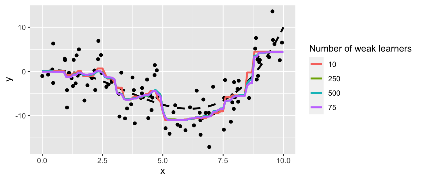

Figure 4.30: Predictions made from the aggregations.

It can be noted that increasing the number of trees smoothes the prediction surface.

What is the effect of increasing the number of trees on the predictive capacities of the model? We can explore this with simulation – again.

First, we need to get some out of sample data.

set.seed(234)
x_new <- runif(n=n, min=0, max=10)
eps <- rnorm(n, 0, 4)
y_new <- f(x)+eps
df_sim_new <- tibble(x=x_new, y=y_new)

We will compute the Mean Squared Error (MSE) on these unseen data. We will do this by varying the number of weak learners, in order to visualise the evolution of the MSE as a function of the number of trees.

mse_test_bagging <- 
  map(1:500, ~add_column(
  df_sim_new, 
  nb_bagg = .,
  pred = predict_bagged(baggin_models_2[1:.], df_sim_new))) %>% 
  map(~mutate(., mse = (y-pred)^2)) %>% 
  map_df(~summarise(., nb_bagg=unique(nb_bagg), mse = mean(mse)))

Then, the results can be plotted.

ggplot(data = mse_test_bagging,
       mapping = aes(x = nb_bagg, y = mse)) +
  geom_line() +
  labs(x = "Number of trees (weak learners)", y = "MSE") +
  theme(plot.title.position = "plot")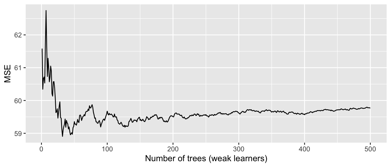

Figure 4.31: MSE vs number of trees.

We can note two things from this graph:

after a certain number of trees used is reached, the MSE seems to stabilise: here, we could use around 150 trees only
using more trees than what would be enough does not lead to overfitting.

4.4.1.2 Out-of-bag estimations

We just had a look at the performance of our models using the validation set approach. Actually, we could have a look at how the model performs on unseen data differently. When a bootstrap sample is used to create a tree, on average, only two third of the observations end up in the sample. Hence, the remaining observations can be used to make out-of-sample predictions. The conventional term for these out-of-sample observations is: out-of-bag observations. Averaging the predicted value of an observation over the learners in which it was out-of-bag gives an out-of-bag prediction. Doing it for all of the observations of the sample allows us to compute the overall out-of-bag MSE.

As the out-of-bag predictions are made on unseen data, the out-of-bag MSE is computed using unseen data and can therefore be used to assess the goodness of fit of the model.

This can easily be implemented with a function. After the unpruned tree is grown, all we need to do is to use it to make predictions on the left-out data. We need to keep track on which data it concerns, though.

train_weak_learner <- function(data, formula, method, control){
  n <- nrow(data)
  ind_x <- sample(1:n, size = n, replace = TRUE)
  df_tmp <- data[ind_x,]
  cart <- rpart(formula = formula, 
                data = df_tmp,
                method = method,
                control = control)
  
  # oob predictions
  oob_pred <- predict(cart, newdata = data[-ind_x,])
  names(oob_pred) <- seq(1,n)[-ind_x]
  
  list(estim = cart, oob_pred = oob_pred)
}

Let us use a loop to build 500 trees.

library(doSNOW)
ncl <- parallel::detectCores()-1
(cl <- makeCluster(ncl))

## groupe de processus socket avec 7 noeuds sur l'hôte 'localhost'

registerDoSNOW(cl)

baggin_models_3 <- foreach(
  i = 1:500,
  .packages=c("rpart")) %dopar% {
  
  train_weak_learner(
    data = df_sim,
    formula = y~x, 
    method="anova", 
    control = rpart.control(cp = 0))
}

stopCluster(cl)

The out-of-bag predictions can the be computed:

oob_pred <- 
  map(baggin_models_3, "oob_pred") %>% 
  map_df(~as_tibble(., rownames = "id")) %>% 
  bind_rows() %>% 
  mutate(id = as.numeric(id)) %>% 
  rename(pred = value) %>% 
  group_by(id) %>% 
  summarise(nb_seen = n(),
            pred = mean(pred))
oob_pred

## # A tibble: 100 × 3
##       id nb_seen   pred
##    <dbl>   <int>  <dbl>
##  1     1     198  -1.47
##  2     2     185  -6.17
##  3     3     180  -5.59
##  4     4     192   2.57
##  5     5     181   4.61
##  6     6     175  -1.00
##  7     7     194 -10.4 
##  8     8     187   3.91
##  9     9     179 -11.3 
## 10    10     194  -4.69
## # … with 90 more rows

Just for the sake of it, we can check how many times each observations has been used as an out-of-bag observation over the 500 trees:

summary(oob_pred$nb_seen)

##    Min. 1st Qu.  Median    Mean 3rd Qu.    Max. 
##   160.0   177.8   182.5   183.6   190.0   205.0

The out-of-bag MSE can then be computed:

df_sim %>% 
  mutate(id = row_number()) %>% 
  left_join(oob_pred) %>% 
  mutate(error_sq = (y-pred)^2) %>% 
  summarise(mse = mean(error_sq))

## # A tibble: 1 × 1
##     mse
##   <dbl>
## 1  15.7

Now, let us make the number of tree vary and look how it affects the out-of-bag MSE. Again, a helper function may be convenient.

#' Computes the OOB MSE using `nb_tree` trees
#' @param nb_tree number of trees used (weak learners)
compute_oob_mse_nb_trees <- function(nb_tree){
  oob_pred <- 
    map(baggin_models_3[1:nb_tree], "oob_pred") %>% 
    map_df(~as_tibble(., rownames = "id")) %>% 
    bind_rows() %>% 
    mutate(id = as.numeric(id)) %>% 
    rename(pred = value) %>% 
    group_by(id) %>% 
    summarise(nb_seen = n(),
              pred = mean(pred))
  
  df_sim %>% 
    mutate(id = row_number()) %>% 
    left_join(oob_pred, by = "id") %>% 
    mutate(error_sq = (y-pred)^2) %>% 
    summarise(mse = mean(error_sq, na.rm=TRUE)) %>% 
    mutate(nb_tree = nb_tree)
}

Let us compute the out-of-bag MSE on models that use from 1 to 300 trees. With a too small number of trees, as all the observations will not necessarily be left-out, computing the mean would result in a NA value, unless we specify that NA values should be discarded before computing the average.

oob_mse_nb_trees <- map_df(1:300, compute_oob_mse_nb_trees)

Let us visualise the results:

ggplot(data = oob_mse_nb_trees,
       mapping = aes(x = nb_tree, y = mse)) +
  geom_line() +
  labs(x = "Number of trees grown (weak learners", y = "MSE") +
  theme(plot.title.position = "plot")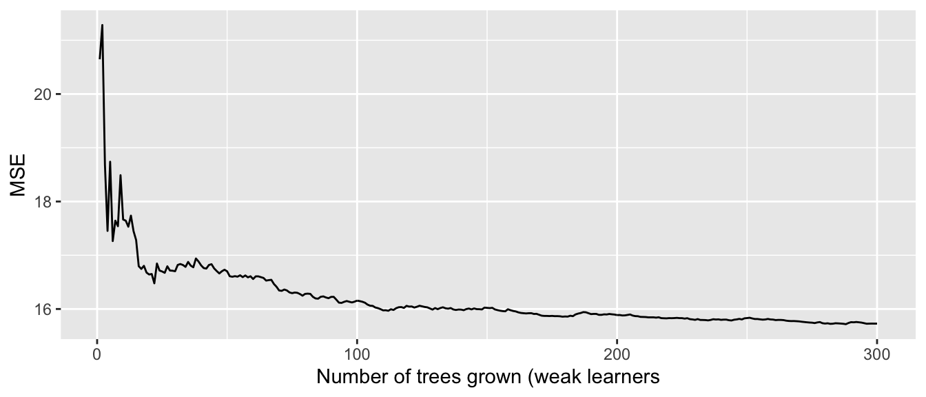

Figure 4.32: Out-of-bag MSE - Bagging.

As in the validation approach, we are able to see with this graph that after a certain number of trees, the error no longer decreases.

4.4.1.3 Variable Importance Measures

To assess the variable importance with bagging, we can proceed in a similar fashion to what we have done with regression or classification trees.

For each tree, we can compute the decrease in the RSS in the case of a regression problem, or the improvement in the Gini impurity index (or Entropy) in the case of a classification problem, for each variable. Then, these values can be averaged over the trees. Again, if the value is large, it hints that the variable is an important predictor.

We can go back to our bike data to illustrate the method. First, we need to grow many unpruned trees.

library(doSNOW)
ncl <- parallel::detectCores()-1
(cl <- makeCluster(ncl))

## groupe de processus socket avec 7 noeuds sur l'hôte 'localhost'

registerDoSNOW(cl)

bagging_models_bike <- foreach(
  i = 1:200,
  .packages=c("rpart", "dplyr")
  ) %dopar% {
  
  train_weak_learner(
    data = df_train %>% select(-y_binary, -date),
    formula = rented_bike_count~., 
    method="anova",
    control = rpart.control(cp = 0))
}

stopCluster(cl)

Then, we can extract the variable importance measures from all these trees, and average the values over the trees:

variable_importance <- 
  map(bagging_models_bike, "estim") %>% 
  map("variable.importance") %>% 
  bind_rows() %>% 
  colMeans()

The relative measure can be computed as follows:

variable_importance_df <- 
  as_tibble(100*variable_importance/sum(variable_importance),
          rownames = "variable")
variable_importance_df

## # A tibble: 14 × 2
##    variable                value
##    <chr>                   <dbl>
##  1 temperature           17.9   
##  2 month                 14.4   
##  3 dew_point_temperature 14.7   
##  4 hour                  15.1   
##  5 seasons               11.2   
##  6 solar_radiation        6.89  
##  7 humidity               6.89  
##  8 rainfall               3.43  
##  9 year                   2.90  
## 10 wind_speed             2.43  
## 11 week_day               1.92  
## 12 visibility             1.95  
## 13 holiday                0.0936
## 14 snowfall               0.126

And we can visualise it using a barplot.

ggplot(data = variable_importance_df,
       mapping = aes(x = value, y = fct_reorder(variable, value))) +
  geom_bar(stat="identity")+
  labs(x = NULL, y = NULL) +
  theme(plot.title.position = "plot")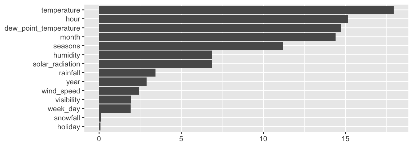

Figure 4.33: Variable relative importance.

4.4.1.4 Pre-built Function

Rather than using the previous codes which are not optimised for fast running, we can use the bagging() function of {ipred}. Having unpacked the method, it is easy to understand the use of this function. First, the package {ipred} can be loaded:

library(ipred)

The number of trees grown is controlled by the argument nbagg. To obtain out-of-bat estimate of the error rate, the coob argument needs to be set to TRUE. The argument control can be fed with a list of values for the different parameters we want for the weak learners. We want to build unpruned trees, so we set cp=0. Then we can play with the other parameters, such as the minimum number of split minsplit (but this may result in pruned trees), the minimum observations in the terminal leaves minbucket, the number of competitor variable we want to retain in the output maxcompete, the number of surrogate splits retained in the output maxsurrogate, etc. Let us just set cp=0 here.

mod_bag <- bagging(
  formula = rented_bike_count ~ .,
  data = df_train %>% select(-y_binary, -date),
  nbagg = 100,  
  coob = TRUE,
  control = rpart.control(cp = 0)
)

The trees are stored in the element mtrees

class(mod_bag$mtrees) ; length(mod_bag$mtrees)

## [1] "list"

## [1] 100

If we look at the first element of mtrees, we can notice that it contains two elements:

bindx: the indices of the observations used to grow the tree (row number of the initial data)
btree: the estimated weak learner

names(mod_bag$mtrees[[1]])

## [1] "bindx" "btree"

head(mod_bag$mtrees[[1]]$bindx)

## [1] 4411  188 1348 1931 4869 2808

The out-of-bag error is stored in the err element. The reported value depends on the type of problem:

for regression problems, it is the root mean squared error (RMSE)
for classification problems, it is the misclassification rate.

mod_bag$err

## [1] 175.0919

The variable importance can be obtained using the methodology we used. But we can also rely on a very convenient package (which will be used afterwards with random forests): {caret}. This package offers a function called varImp().

library(caret)
variable_importance <- varImp(mod_bag)
variable_importance

##                         Overall
## dew_point_temperature 66.062358
## holiday                2.583719
## hour                  55.000256
## humidity              60.226333
## month                 44.683457
## rainfall               7.881722
## seasons               13.489418
## snowfall               5.235853
## solar_radiation       41.959113
## temperature           77.962421
## visibility            53.343140
## week_day              69.950691
## wind_speed            46.141727
## year                   6.792069

And once again the values can be plotted on a barplot:

ggplot(data = as_tibble(variable_importance, rownames = "variable"),
       mapping = aes(x = Overall, y = fct_reorder(variable, Overall))) +
  geom_bar(stat="identity")+
  labs(x = NULL, y = NULL) +
  theme(plot.title.position = "plot")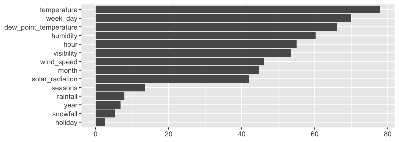

Figure 4.34: Variable relative importance.

4.4.2 Random Forests

The idea behind random forest is very similar to what is done with bagging. Many decision trees are build using bootstrapped training samples, but instead of considering all the variables as candidates each time a split is attempted, only a random sample of the explanatory variables is considered (Leo Breiman 2001). Proceeding this way allows to decorrelate the trees. In fact, with bagging, the trees grown are not completely independent.

If wee look at the top of the first trees grown using bagging, we can notice that the variables used to make the first splits is often the same, and the cutoff is also often very similar, despite the fact that the observations were randomly drawn to create bootstrap training samples:

tree_1_pruned <- prune(mod_bag$mtrees[[1]]$btree, cp=.1)
tree_2_pruned <- prune(mod_bag$mtrees[[2]]$btree, cp=.1)
tree_3_pruned <- prune(mod_bag$mtrees[[3]]$btree, cp=.1)
tree_4_pruned <- prune(mod_bag$mtrees[[4]]$btree, cp=.1)

op <- par()
par(mfrow = c(2,2))
rpart.plot(tree_1_pruned, main = "Tree 1")
rpart.plot(tree_2_pruned, main = "Tree 2")
rpart.plot(tree_3_pruned, main = "Tree 3")
rpart.plot(tree_4_pruned, main = "Tree 4")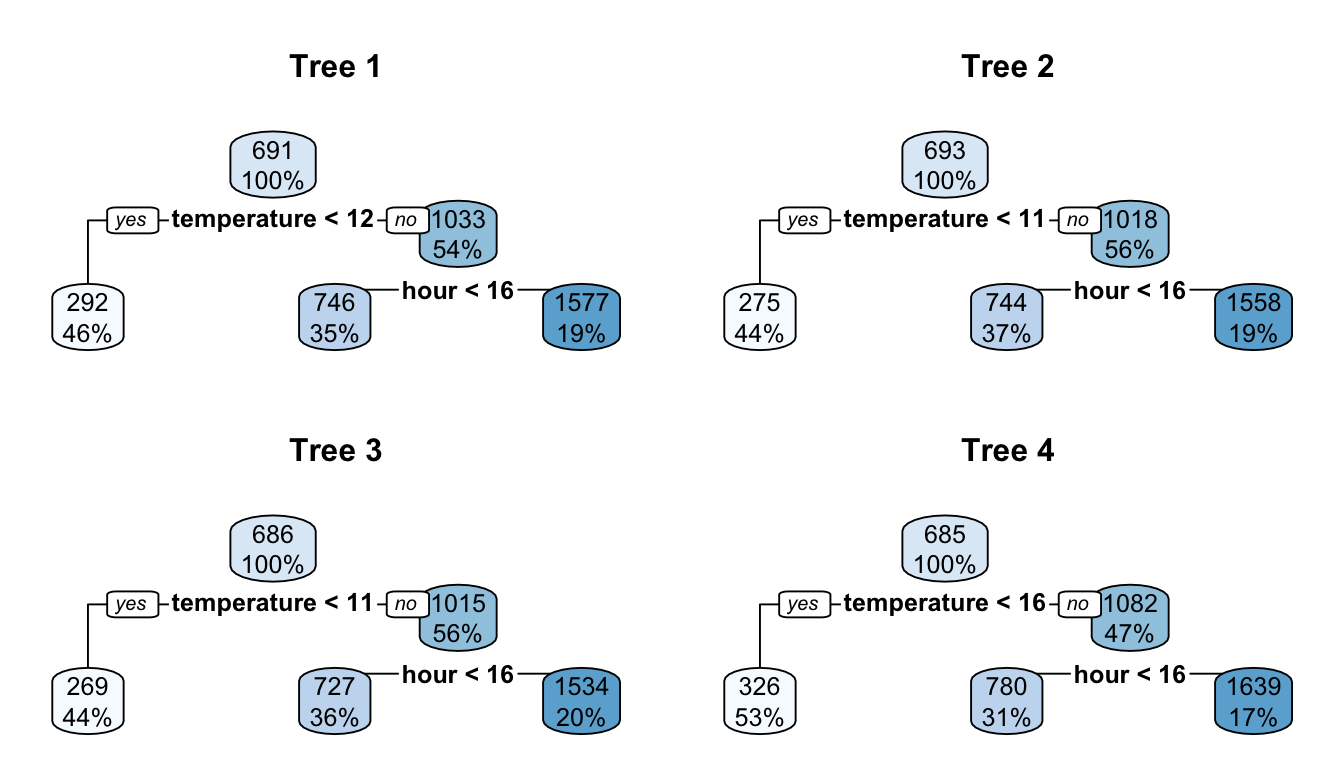

Figure 4.35: Trees may be correlated when use bagging.

par(op)

By sampling $m$ variables among the $p$ predictors so that the former are considered as competitors to make a split, random forests overcome this pitfall. Averaging the predictions made on decorellated trees will produce better results, with less variance.

Default values for the number of variables randomly samples as competitors/candidates at each split are usually :

$m=p/3$ for regression problems
$m=\sqrt{p}$ for classification problems.

4.4.2.1 A First Example with {randomForest}

The package {randomForest} provides a function called randomForest() which implements Breiman’s random forest algorithm for classification and regression. Let us see how to use that function. First, the package can be loaded.

library(randomForest)

The formula and the data arguments can once again be used. Other arguments allow us to tune the algorithm:

ntree: number of trees to grow
mtry: number of variables randomly sampled as candidates at each split.
nodesize: minimum size of terminal nodes. The default value is:
- 1 for classification problems
- 5 for regressio problems
maxnodes: maximum number of terminal nodes trees in the forest can have. If not given, trees are grown to the maximum possible (subject to limits by nodesize). If set larger than maximum possible, a warning is issued.

Let us grow 200 trees and set the number of variables randomly sampled as candidates at each split ($m$) to 5, i.e., the square root of our number of predictors. We will define nodesize and maxnodes with their default values.

mod_rf <- 
  randomForest(
  formula = rented_bike_count ~ .,
  data = df_train %>% select(-y_binary, -date),
  ntree = 200,
  mtry = round(ncol(select(df_train, -y_binary, -date))/3),
  nodesize = 5,
  maxnodes = NULL
)

The out-of-bag MSE computed using 1 to 100 trees are stored in the mse elements of the model:

df_plot_mse_oob_rf <- 
  tibble(mse = mod_rf$mse) %>% 
  mutate(nb_tree = row_number())
df_plot_mse_oob_rf

## # A tibble: 200 × 2
##       mse nb_tree
##     <dbl>   <int>
##  1 95175.       1
##  2 88586.       2
##  3 82743.       3
##  4 70951.       4
##  5 66796.       5
##  6 62666.       6
##  7 59989.       7
##  8 56013.       8
##  9 53375.       9
## 10 51505.      10
## # … with 190 more rows

For comparison, let us compute the MSE obtained on a test sample. We can use the predict() function from {randomForest} to get the predicted values for all the trees, using the out-of-bag sample (to my understanding, it is not possible to directly ask for the predictions made using a single tree).

predictions_test_tree_wise <- 
  predict(mod_rf, newdata = df_test, predict.all = TRUE)

The individual element of the returned object contains a matrix with the predicted values. Each column corresponds to the estimated values of a single tree.

dim(predictions_test_tree_wise$individual)

## [1] 1693  200

All we need to do is to compute the MSE using up to nb_tree:

#' Computes the MSE using `nb_tree` trees
compute_mse_trees <- function(nb_tree){
  pred <- predictions_test_tree_wise$individual[,1:nb_tree]
  if(nb_tree > 1) pred <- rowMeans(pred)
  tibble(mse = mean((df_test$rented_bike_count - pred)^2), 
         nb_tree = nb_tree)
}

df_plot_mse_test_rf <- map_df(1:200, compute_mse_trees)
df_plot_mse_test_rf

## # A tibble: 200 × 2
##        mse nb_tree
##      <dbl>   <int>
##  1 336998.       1
##  2 246233.       2
##  3 232757.       3
##  4 194906.       4
##  5 167375.       5
##  6 163933.       6
##  7 161718.       7
##  8 161246.       8
##  9 158161.       9
## 10 157843.      10
## # … with 190 more rows

For the sake of comparison, let us compare these MSE to that obtained with bagging.

mod_bag <- bagging(
  formula = rented_bike_count ~ .,
  data = df_train %>% select(-y_binary, -date),
  nbagg = 200,  
  coob = TRUE,
  control = rpart.control(cp = 0)
)

Let us first compute the out-of-bag MSE.

#' Computes out-ob-bag predictions for the ith tree
compute_oob_bagging <- function(i, model, data){
  n <- nrow(data)
  current_tree <- model$mtrees[[i]]$btree
  ind_x_current <- model$mtrees[[i]]$bindx
  oob_pred <- predict(current_tree, newdata = data[-ind_x_current,])
  as_tibble(oob_pred) %>% 
    mutate(ind_x = seq(1,n)[-ind_x_current], tree = i)
}

oob_bagging <- 
  map_df(1:length(mod_bag$mtrees), 
         ~compute_oob_bagging(.,mod_bag, df_train))
oob_bagging

## # A tibble: 497,933 × 3
##    value ind_x  tree
##    <dbl> <int> <int>
##  1 390.     10     1
##  2 439.     14     1
##  3 405      17     1
##  4 412.     18     1
##  5 418      20     1
##  6 342.     24     1
##  7 277      25     1
##  8 248.     27     1
##  9  74.9    31     1
## 10 306.     35     1
## # … with 497,923 more rows

Based on those out-of-bags predictions, we can compute the out-of-bag overall MSE depending on how many trees are considered:

#' Computes out-of-bag MSE using out-of-bag predictions
#' from `nb_tree` trees
compute_mse_oob_ntree <- function(nb_tree){
  
  oob_pred <- 
    oob_bagging %>% 
    filter(tree <= nb_tree) %>% 
    group_by(ind_x) %>% 
    summarise(oob_pred = mean(value))
  
  df_train %>% 
    mutate(ind_x = row_number()) %>% 
    left_join(
      oob_pred,
       by = "ind_x"
    ) %>% 
    mutate(error_sq = (rented_bike_count-oob_pred)^2) %>% 
    summarise(mse = mean(error_sq, na.rm=TRUE)) %>% 
    mutate(nb_tree = nb_tree)
  
}

df_plot_mse_oob_bagging <- 
  map_df(1:length(mod_bag$mtrees), compute_mse_oob_ntree)
df_plot_mse_oob_bagging

## # A tibble: 200 × 2
##       mse nb_tree
##     <dbl>   <int>
##  1 51984.       1
##  2 53239.       2
##  3 47821.       3
##  4 46944.       4
##  5 44856.       5
##  6 43811.       6
##  7 43563.       7
##  8 42060.       8
##  9 39683.       9
## 10 39366.      10
## # … with 190 more rows

Then, let us finally compute the MSE on a test set. Let us define a helper function that computed the predictions on the test set for the ith tree grown.

#' Computes predictions for the ith tree
#' (helper function)
compute_pred_tree <- function(i, model, newdata){
  current_tree <- model$mtrees[[i]]$btree
  pred <- predict(current_tree, newdata = newdata)
  as_tibble(pred, rownames = "ind_x") %>%
    mutate(tree = i)
}

pred_test_bagging <-
  map_df(1:length(mod_bag$mtrees), 
         ~compute_pred_tree(., mod_bag, df_test))

The MSE on the test set:

#' Compute the MSE on a test set (`df_test`)
#' @param nb_tree number of trees used to compute the MSE
compute_mse_bagging_ntree <- function(nb_tree){

  pred <-
    pred_test_bagging %>%
    mutate(ind_x = as.numeric(ind_x)) %>%
    filter(tree <= nb_tree) %>%
    group_by(ind_x) %>%
    summarise(oob_pred = mean(value))

  df_train %>%
    mutate(ind_x = row_number()) %>%
    left_join(
      pred,
      by = "ind_x"
    ) %>%
    mutate(error_sq = (rented_bike_count-oob_pred)^2) %>%
    summarise(mse = mean(error_sq, na.rm=TRUE)) %>%
    mutate(nb_tree = nb_tree)

}
df_plot_mse_test_bagging <- 
  map_df(1:length(mod_bag$mtrees), compute_mse_bagging_ntree)
df_plot_mse_test_bagging

## # A tibble: 200 × 2
##        mse nb_tree
##      <dbl>   <int>
##  1 633941.       1
##  2 594158.       2
##  3 580209.       3
##  4 595718.       4
##  5 601718.       5
##  6 606807.       6
##  7 602178.       7
##  8 599957.       8
##  9 605989.       9
## 10 613597.      10
## # … with 190 more rows

We now have:

df_plot_mse_oob_bagging: out-of-bag MSE for bagging
df_plot_mse_test_bagging: MSE computed on the test set for bagging
df_plot_mse_oob_rf: out-of-bag MSE for random forest
df_plot_mse_test_rf: MSE computed on the test set for random forest

Let us plot those errors:

df_plot <- 
  df_plot_mse_oob_bagging %>% 
  mutate(type = "OOB", model = "Bagging") %>% 
  bind_rows(
    df_plot_mse_test_bagging %>% 
      mutate(type = "Test", model = "Bagging")
  ) %>% 
  bind_rows(
    df_plot_mse_oob_rf %>% 
      mutate(type = "OOB", model = "Random Forests")
  ) %>% 
  bind_rows(
    df_plot_mse_test_rf %>% 
      mutate(type = "Test", model = "Random Forests")
  )

ggplot(data = df_plot,
       mapping = aes(x = nb_tree, y = mse)) +
  geom_line(mapping = aes(colour = model)) +
  labs(x = "Number of trees", y = "Error (MSE)") +
  theme(plot.title.position = "plot") +
  facet_wrap(~type, scales = "free_y", ncol = 2)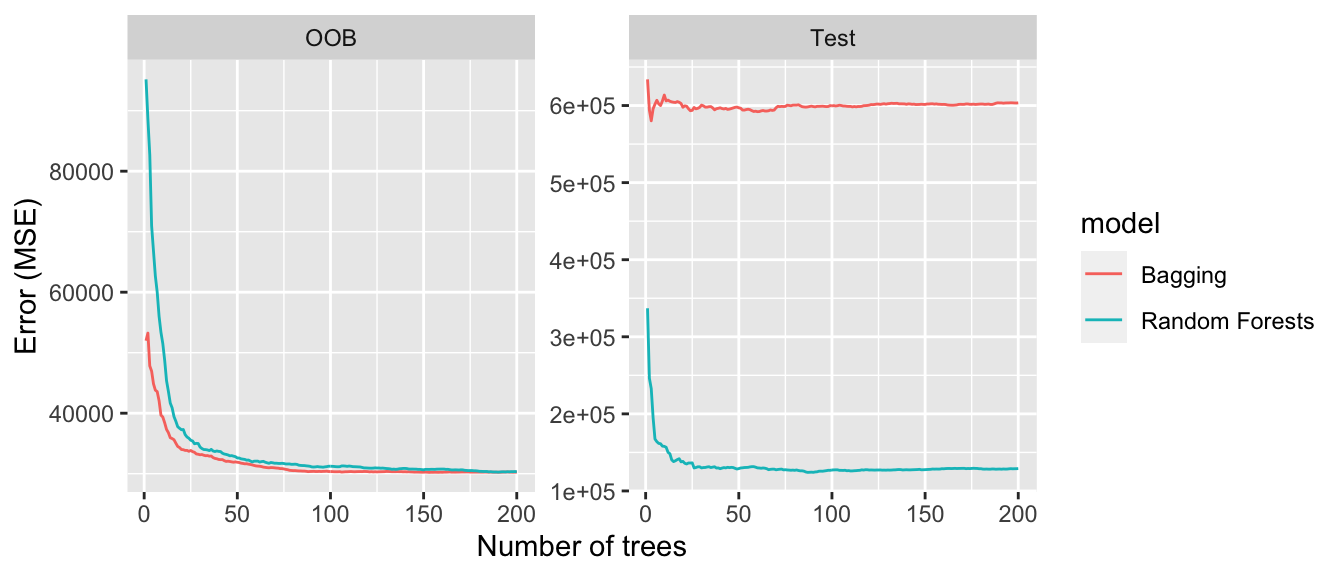

Figure 4.36: Goodness of fit depending on the number of trees.

We note that the OOB error are lower than the errors computed on the test set.

The errors obtained with a Random Forest are usually lower than their counterpart obtained with bagging (which is not the case here!).

4.4.2.2 Varying the hyperparameters

We have just seen in the last graph that the error of the model seem to stabilize after a certain number of trees. If the number of trees is too large, it causes no overfitting, it just takes longer to estimate the model.

4.4.2.2.1 Varying `mtry`

Let us make the hyperparameter mtry that controls the number of variables sampled from the predictors to perform a split. We will consider values ranging from 1 to 5. In each case, we will grow a random forest, and then look at the out-of-bag error depending on the number of trees grown.

library(doSNOW)
ncl <- parallel::detectCores()-1
(cl <- makeCluster(ncl))

## groupe de processus socket avec 7 noeuds sur l'hôte 'localhost'

registerDoSNOW(cl)

# With a progress bar
# pb <- txtProgressBar(min=1, max = 5, style = 3)
# progress <- function(n) setTxtProgressBar(pb, n)
# opts <- list(progress = progress)

nb_predictors <- ncol(df_train %>% select(-y_binary, -date))

mod_rf_mtry <- foreach(
  mtry=1:5,
  .packages=c("randomForest", "dplyr")
  # .options.snow = opts) %dopar% { # With probressbar
  ) %dopar% {
    randomForest(
      formula = rented_bike_count ~ .,
      data = df_train %>% select(-y_binary, -date),
      ntree = 200,
      mtry = mtry,
      nodesize = 5,
      maxnodes = NULL
    )
  }
# close(pb)
stopCluster(cl)

From the results, we can extract the out-of-bag MSE:

df_plot_mtry <- 
  map(mod_rf_mtry, "mse") %>% 
  map_df(~tibble(mse=.) %>% 
           mutate(nb_tree = row_number()), .id = "mtry")
df_plot_mtry

## # A tibble: 1,000 × 3
##    mtry      mse nb_tree
##    <chr>   <dbl>   <int>
##  1 1     296754.       1
##  2 1     267732.       2
##  3 1     251870.       3
##  4 1     225596.       4
##  5 1     212433.       5
##  6 1     210395.       6
##  7 1     201370.       7
##  8 1     185925.       8
##  9 1     171962.       9
## 10 1     172937.      10
## # … with 990 more rows

And then we can plot the results:

ggplot(data = df_plot_mtry,
       mapping = aes(x = nb_tree, y = mse)) +
  geom_line(mapping = aes(colour = mtry)) +
  labs(x = "Number of trees", y = "Error (MSE)")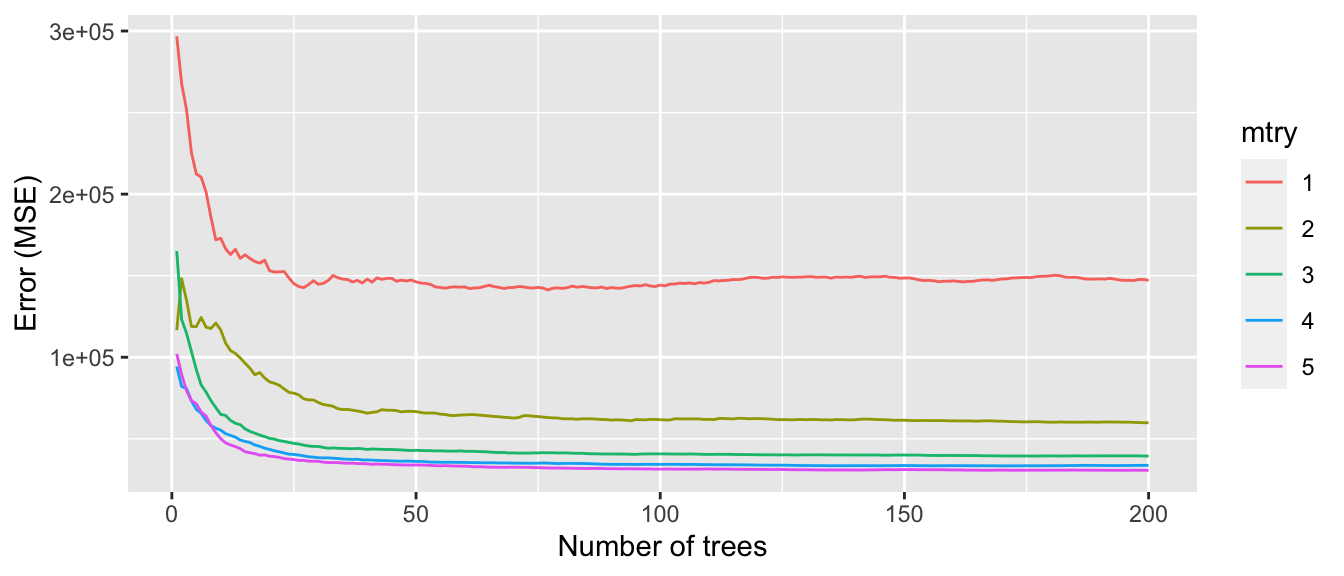

Figure 4.37: Varying the number of variables samples to perform a split.

Recall that taking only a random sample of $m$ variables among the $p$ available to perform a split allows us to decorrelate the trees. Boehmke and Greenwell (2019) notes that in the presence of a lot of noise in the data, when there are few predictors, high values for mtry allow the selection of variables with a stronger signal. On the other hand, when there are many relevant predictors, low values of mtry offer better performance. In practice, it is therefore necessary to test multiple values in order to select the one that offers the most interesting results in terms of error reduction.

We will see in a subsequent section how to create a grid search that allows to fine tune the model. In other words, we will create a matrix that will contain combinations of different values for the hyperparameters of the model (a grid) and we will iterate over that grid to try each possible combination contained in it.

4.4.2.2.2 Varying `nodesize`

Let us now consider varying the minimum size of terminal nodes. Recall that increasing the numner of nodesize leads to smaller trees (which thus fastens the computation).

library(doSNOW)
ncl <- parallel::detectCores()-1
(cl <- makeCluster(ncl))

## groupe de processus socket avec 7 noeuds sur l'hôte 'localhost'

registerDoSNOW(cl)

# pb <- txtProgressBar(min=1, max = 4, style = 3)
# progress <- function(n) setTxtProgressBar(pb, n)
# opts <- list(progress = progress)

nb_predictors <- ncol(df_train %>% select(-y_binary, -date))


mod_rf_nodesize <- foreach(
  nodesize = c(5, 10, 15, 20),
  .packages=c("randomForest", "dplyr")
  # .options.snow = opts # progressbar
  ) %dopar% {
    randomForest(
      formula = rented_bike_count ~ .,
      data = df_train %>% select(-y_binary, -date),
      ntree = 200,
      mtry = round(nb_predictors/3),
      nodesize = nodesize,
      maxnodes = NULL
    )
  }
# close(pb)
stopCluster(cl)

The out-of-bag errors can once again be extracted from the different models:

df_plot_nodesize <- 
  map(mod_rf_nodesize, "mse") %>% 
  map_df(~tibble(mse=.) %>% mutate(nb_tree = row_number()), .id = "ind_nodesize") %>% 
  mutate(ind_nodesize = as.numeric(ind_nodesize)) %>% 
  left_join(
    tibble(nodesize = c(5, 10, 15, 20)) %>% mutate(ind_nodesize = row_number()),
    by = "ind_nodesize"
  )

df_plot_nodesize

## # A tibble: 800 × 4
##    ind_nodesize     mse nb_tree nodesize
##           <dbl>   <dbl>   <int>    <dbl>
##  1            1 107488.       1        5
##  2            1  91532.       2        5
##  3            1  87385.       3        5
##  4            1  81312.       4        5
##  5            1  70797.       5        5
##  6            1  68423.       6        5
##  7            1  64530.       7        5
##  8            1  59660.       8        5
##  9            1  56389.       9        5
## 10            1  53079.      10        5
## # … with 790 more rows

And then we can plot the results:

ggplot(data = df_plot_nodesize,
         mapping = aes(x = nb_tree, y = mse)) +
  geom_line(mapping = aes(colour = factor(nodesize))) +
  labs(x = "Number of trees", y = "Error (MSE)") +
  scale_colour_discrete("nodesize")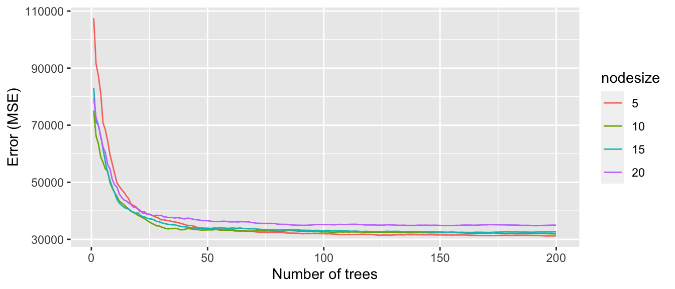

Figure 4.38: Varying the minimum size of terminal nodes.

Once again, we need to loop over different values to try to find the one that will produce the best results.

4.4.2.2.3 Varying `maxnodes`

Lastly, let us consider the argument maxnodes that controls the maximum number of terminal nodes trees in the forest can have. If the value is not provided, as was the case in all our other examples, trees are grown to the maximum possible (subject to limits by nodesize).

library(doSNOW)
ncl <- parallel::detectCores()-1
(cl <- makeCluster(ncl))

## groupe de processus socket avec 7 noeuds sur l'hôte 'localhost'

registerDoSNOW(cl)

# pb <- txtProgressBar(min=1, max = 6, style = 3)
# progress <- function(n) setTxtProgressBar(pb, n)
# opts <- list(progress = progress)

nb_predictors <- ncol(df_train %>% select(-y_binary, -date))

mod_rf_maxnodes <- foreach(
  max_nodes = c(5, 10, 20, 30, 40, 50),
  .packages=c("randomForest", "dplyr")
  # .options.snow = opts # with progressbar
  ) %dopar% {
    randomForest(
      formula = rented_bike_count ~ .,
      data = df_train %>% select(-y_binary, -date),
      ntree = 500,
      mtry = round(nb_predictors/3),
      nodesize = 5,
      maxnodes = max_nodes
    )
  }
# close(pb)
stopCluster(cl)

Let us extract the out-of-bag MSE:

df_plot_maxnodes <- 
  map(mod_rf_maxnodes, "mse") %>% 
  map_df(~tibble(mse=.) %>%
           mutate(nb_tree = row_number()), .id = "ind_maxnodes") %>% 
  mutate(ind_maxnodes = as.numeric(ind_maxnodes)) %>% 
  left_join(
    tibble(maxnodes = c(5, 10, 20, 30, 40, 50)) %>% 
      mutate(ind_maxnodes = row_number()),
    by = "ind_maxnodes"
  )
df_plot_maxnodes

## # A tibble: 3,000 × 4
##    ind_maxnodes     mse nb_tree maxnodes
##           <dbl>   <dbl>   <int>    <dbl>
##  1            1 196418.       1        5
##  2            1 213756.       2        5
##  3            1 221440.       3        5
##  4            1 230535.       4        5
##  5            1 212261.       5        5
##  6            1 217891.       6        5
##  7            1 218916.       7        5
##  8            1 213289.       8        5
##  9            1 208396.       9        5
## 10            1 204294.      10        5
## # … with 2,990 more rows

df_plot_maxnodes

## # A tibble: 3,000 × 4
##    ind_maxnodes     mse nb_tree maxnodes
##           <dbl>   <dbl>   <int>    <dbl>
##  1            1 196418.       1        5
##  2            1 213756.       2        5
##  3            1 221440.       3        5
##  4            1 230535.       4        5
##  5            1 212261.       5        5
##  6            1 217891.       6        5
##  7            1 218916.       7        5
##  8            1 213289.       8        5
##  9            1 208396.       9        5
## 10            1 204294.      10        5
## # … with 2,990 more rows

And plot the results:

ggplot(data = df_plot_maxnodes,
       mapping = aes(x = nb_tree, y = mse)) +
  geom_line(mapping = aes(colour = factor(maxnodes))) +
  labs(x = "Number of trees", y = "Error (MSE)") +
  scale_colour_discrete("maxnodes")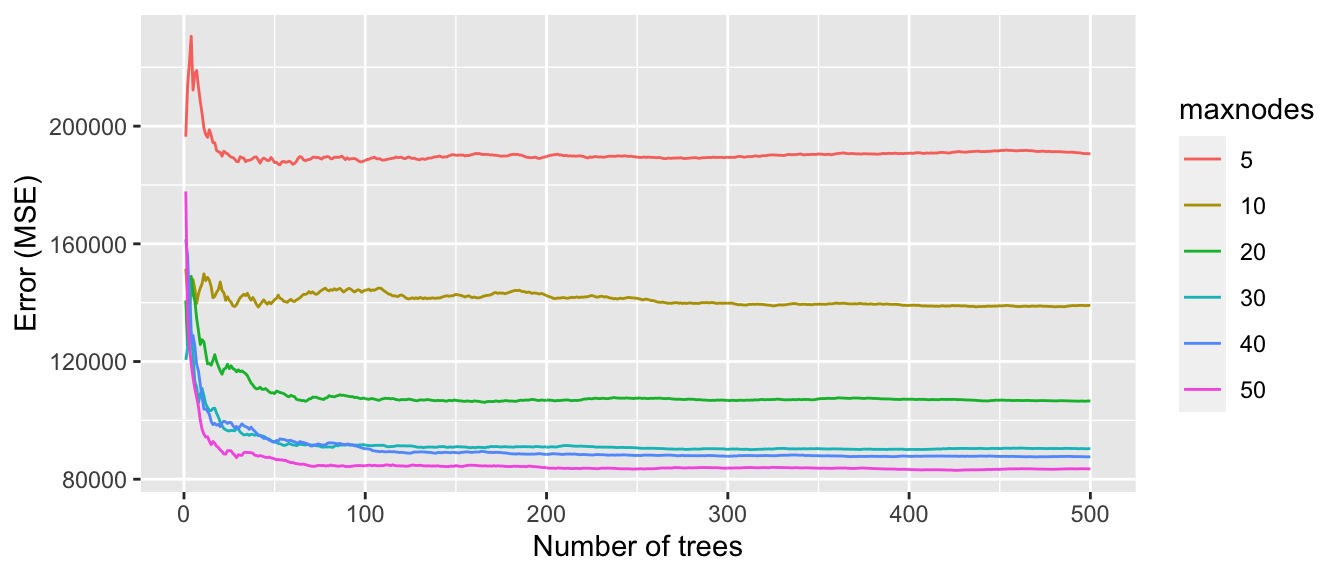

Figure 4.39: Varying the maximum number of terminal nodes trees.

When the number of maximum number of terminal nodes is restricted, it leads to shallower trees. Recall that using unpruned trees creates more sensible weak learners.

4.4.2.3 Variable importance

To get an idea of the importance of the variables, it is possible to rely on the same measures as before, namely the average total reduction in measurement error contributed by each variable. However, Terence Parr, Kerem Turgutlu, Christopher Csiszar, and Jeremy Howard warn us that this default method to compute variable importance is biased (see their notebook). Quoting them:

We’ve known for years that this common mechanism for computing feature importance is biased; i.e. it tends to inflate the importance of continuous or high-cardinality categorical variables.

Another measure is widely used with random forests. It is based on the permutation of variables. The procedure is as follows:

For tree $t \in \{1, \ldots, \text{ntree}\}$, using the out-of-bag sample, compute the goodness of fit (e.g., the MSE for regression problems, or the accuracy for classification problems) : $r^{(t)}$
- For each predictor $j \in \{1,\ldots, p\}$ :
  - generate a new matrix of predictors by permuting predictor $j$ in the matrix of predictors $\mathbf{x}$
  - compute the goodness of fit using the predictions made with the prermuted data: $r_{j}^{(t)}$
  - compute the permutation variable importance for the tree as either:
    - $\text{PI}_{j}^{(t)} =r_{j}^{(t)} - r^{(t)}$
    - $\text{PI}_{j}^{(t)} =\frac{r_{j}^{(t)}}{r^{(t)}}$.
Once the tree-wise permutation importance is estimated for all trees $t$, for each predictor $j \in \{1,\ldots, p\}$ :
- compute the forest-wise permutation importance as the average over all tree-wise permutation importance:
\[\text{PI}_{j} = \frac{\sum_{t=1}^{\text{ntree}} \text{PI}_{j}^{(t)}}{\text{ntree}}.\]

The idea behind this procedure is as follows, as indicated in Debeer and Strobl (2020). If the response variable $y$ and an explanatory variable $\mathbf{x}_j$ have a structural dependence, adding noise to the variable $\mathbf{x}_j$ should destroy this structural dependence. Once the noise is added, the splits made from $\mathbf{x}_j$ become random splits. The contribution of the variable to the decrease in the error criterion/impurity measure (MSE or Gini criterion) should therefore be diminished or even lost. Swapping the values of $\mathbf{x}_j$ is a way of noising this variable. Comparing the goodness of fit of the tree (and the random forest) before and after the noising allows us to quantify the importance of variable $\mathbf{x}_j$ in predicting the response $y$: if the permutation had no effect, the variable $\mathbf{x}_j$ does not matter. If, on the other hand, the permutation results in a decrease in the predictive capacity of the model, then the variable $\mathbf{x}_j$ is important for predicting $y$.

In a first place, we need an estimated random forest. As we will need it for the sake of the illustration, we will keep the out-of-bag errors in the resulting object, setting keep.inbag = TRUE. We will also specifically ask for the default importance metric to be return by setting importance = TRUE.{R}.

mod_rf <- 
  randomForest(
    formula = rented_bike_count ~ .,
    data = df_train %>% select(-y_binary, -date),
    ntree = 100,
    mtry = round(ncol(select(df_train, -y_binary, -date))/3),
    nodesize = 5,
    maxnodes = NULL,
    keep.inbag = TRUE,
    importance = TRUE
  )

Let us define (one again) a function to compute the Mean Squarred Error (we face a regression problem here).

compute_mse <- function(observed, predicted){
  mean((observed-predicted)^2)
}

Let us illustrate how the method works with a single tree and a single noised-up predictor in a first place. We will extend the methodology to get an overall measure afterwards. Let us focus on the first weak learner:

tree_number <- 1

We want to compute the MSE based on the out-of-bag sample for that tree. To get the out-of-bag observations from the first tree, we can proceed as follows:

ind_x_oob <- 
  mod_rf$inbag[, tree_number][mod_rf$inbag[, tree_number] == 0] %>% 
  names() %>% 
  as.numeric()

df_oob <- df_train[ind_x_oob, ]

Let us focus on the first predictor:

predictor_names <- attr(mod_rf$terms, "term.labels")
j <- 1
predictor_names[j]

## [1] "hour"

We can use the predict() function from {randomForest} as we did previously.

predictions_init <- 
  predict(mod_rf, newdata = df_oob, predict.all = TRUE)

Then we can extract only the predicted values from the first tree, and compute the initial MSE, i.e., the MSE computed without noising up the first predictor.

predictions_init_t <- predictions_init$individual[, tree_number]
mse_init_t <- compute_mse(df_oob$rented_bike_count, predictions_init_t)
mse_init_t

## [1] 78511.54

Then, using the sample() fuction, we can noise-up the first predictor.

df_oob_noised_j <- df_oob %>% 
  mutate(!!sym(predictor_names[j]) := 
           sample(!!sym(predictor_names[j]), replace=FALSE))

We can have a glance at the first observations before and after the shuffling:

cbind(init = df_oob[[predictor_names[j]]], 
      noised = df_oob_noised_j[[predictor_names[j]]]) %>% 
  head()

##      init noised
## [1,]    0      8
## [2,]    1      9
## [3,]    4      1
## [4,]    9     20
## [5,]   10     22
## [6,]   21     21

The out-of-bag MSE with this noised-up data can then be computed:

predictions_xj <-
  predict(mod_rf, newdata = df_oob_noised_j, predict.all = TRUE)
predictions_noised_j_t <- 
  predictions_xj$individual[, tree_number]
mse_noised_j_t <- 
  compute_mse(df_oob_noised_j$rented_bike_count, predictions_noised_j_t)
mse_noised_j_t

## [1] 350665.2

cbind(mse_before = mse_init_t, mse_after = mse_noised_j_t)

##      mse_before mse_after
## [1,]   78511.54  350665.2

The MSE greatly rose. But we need to see if this happens with all the trees, and not just with the first one.

Let us define a function that recreate the out-of-bag data for a given tree:

get_oob_data <- function(tree_number, model){
  # Indices of out-of-bag observations
  ind_x_oob <- 
    mod_rf$inbag[, tree_number][model$inbag[, tree_number] == 0] %>% 
    names() %>% 
    as.numeric()
  
  # oob data
  df_train[ind_x_oob, ]
}

Now, we can wrap-up the previous code to expand the computation to all trees and all variables:

#' Computes tree-wise permutation importance
#' @param tree_number index of the t-th tree
#' @param model object of class randomForest
compute_pi_tree <- function(tree_number, model){
  
  # Out-of-bag data for tree `tree_number`
  df_oob <- get_oob_data(tree_number, model)
  
  # tree-wise oob MSE before noising-up predictors
  predictions_init <- predict(model, newdata = df_oob, predict.all = TRUE)
  predictions_init_t <- predictions_init$individual[, tree_number]
  mse_init_t <- compute_mse(df_oob$rented_bike_count, predictions_init_t)
  
  predictor_names <- attr(mod_rf$terms, "term.labels")
  
  # Looping over indices of predictors
  mse_noised_t <- rep(NA, length(predictor_names))
  for(j in seq_along(predictor_names)){
    # Noising-up data
    df_oob_noised_j <- df_oob %>% 
      mutate(!!sym(predictor_names[j]) := sample(
        !!sym(predictor_names[j]),
        replace=FALSE))
    
    # tree-wise oob MSE after noising-up jth predictor
    predictions_xj <- 
      predict(model, newdata = df_oob_noised_j, predict.all = TRUE)
    predictions_noised_j_t <- 
      predictions_xj$individual[, tree_number]
    mse_noised_j_t <- 
      compute_mse(df_oob_noised_j$rented_bike_count, predictions_noised_j_t)
    mse_noised_t[[j]] <- mse_noised_j_t
  }
  
  # tree-wise permutation importance
  tree_wise_pi <- mse_noised_t-mse_init_t
  names(tree_wise_pi) <- predictor_names
  tree_wise_pi
}

The tree-wise permutation importance of the variables computed over the first tree can be obtained as follows:

permutation_importance_t <- compute_pi_tree(tree_number = 1, model = mod_rf)
permutation_importance_t

##                  hour           temperature              humidity 
##          2.766762e+05          2.947449e+05          5.654866e+04 
##            wind_speed            visibility dew_point_temperature 
##          7.344090e+03          5.761622e+03          1.604150e+04 
##       solar_radiation              rainfall              snowfall 
##          1.111862e+05          2.516485e+04          5.721013e+02 
##               seasons               holiday                  year 
##          1.649556e+04          1.017557e+03         -8.320239e-02 
##                 month              week_day 
##          2.768299e+04          4.095305e+04

The tree-wise permutation importance values for all trees can then be obtained by looping over the trees:

tree_wise_pi <- 
  map(1:mod_rf$ntree, ~compute_pi_tree(., model = mod_rf))

The results can be put in a table:

tree_wise_pi_df <- 
  tree_wise_pi %>% 
  map_df(~as_tibble(., rownames = "variable"), .id="tree")
tree_wise_pi_df

## # A tibble: 1,400 × 3
##    tree  variable                value
##    <chr> <chr>                   <dbl>
##  1 1     hour                  281244.
##  2 1     temperature           286672.
##  3 1     humidity               62440.
##  4 1     wind_speed              4406.
##  5 1     visibility              4968.
##  6 1     dew_point_temperature  14472.
##  7 1     solar_radiation       126512.
##  8 1     rainfall               28872.
##  9 1     snowfall                 739.
## 10 1     seasons                15761.
## # … with 1,390 more rows

Lastly, the forest-wise permutation importance of each variable can be calculated:

permutation_importance <- 
  tree_wise_pi_df %>% 
  group_by(variable) %>% 
  summarise(permutation_importance = mean(value)) %>% 
  arrange(desc(permutation_importance))

These can be visualised over a barplot:

ggplot(data = permutation_importance,
       mapping = aes(x = permutation_importance,
                     y = fct_reorder(variable, permutation_importance))) +
  geom_bar(stat = "identity") +
  labs(x = "Permutation importance", y = NULL)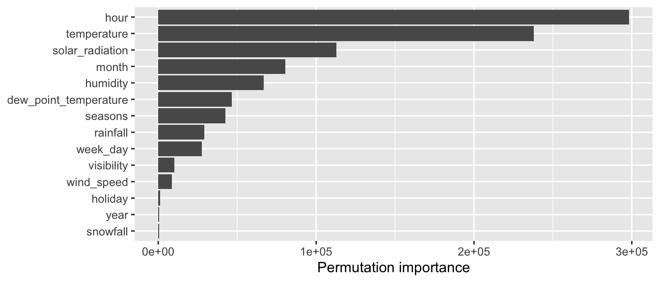

Figure 4.40: Tree-wise permutation importance.

For comparison, we can have a loop at the variable importance as computed with the standard method:

ggplot(data = as_tibble(mod_rf$importance, rownames = "variable"),
       mapping = aes(x = IncNodePurity,
                     y = fct_reorder(variable, IncNodePurity))) +
  geom_bar(stat = "identity") +
  labs(x = "Variable importance (Increase in node Purity)", y = NULL)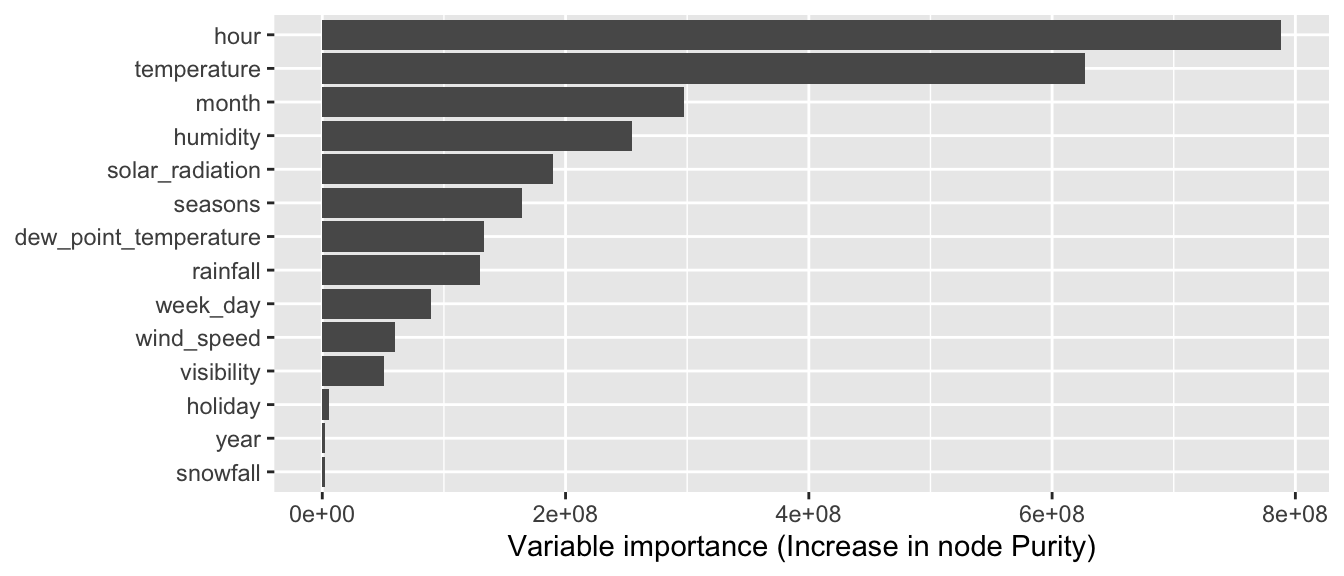

Figure 4.41: Variable importance: default method computed using the increase in node purity.

We note a few changes.

Obviously, to obtain the forest-wise permutation importance, there already exists a pre-build function in {randomForest}: importance().

# Permutation importance
imp <- importance(mod_rf, type=1, scale = F)

ggplot(data = as_tibble(imp, rownames = "variable"),
       mapping = aes(x = `%IncMSE`,
                     y = fct_reorder(variable, `%IncMSE`))) +
  geom_bar(stat = "identity") +
  labs(x = "Permutation importance (% Increase in MSE)", y = NULL)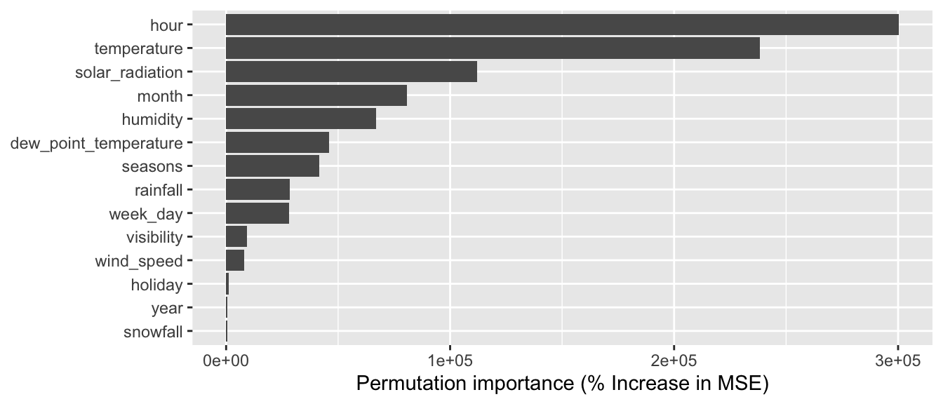

Figure 4.42: Permutation importance returned by randomForest: percent increase in MSE.

4.4.2.4 Fine Tuning

We have seen that some hyperparameters of the random forest can be changed. Tweaking those hyperparameters may affect greatly the predictive capacities of the model.

We have seen that when we increase the number of trees to be grown, the MSE stabilises. Having too many trees does not cause overfitting. Boehmke and Greenwell (2019) suggests the following rule of thumb to pick a first value for the number of trees to be grown: 10 times the number of predictors.

In our Seoul bikes dataset, the number of predictors is:

number_predictors <- 
  df_train %>% select(-y_binary, -date) %>% ncol()
number_predictors

## [1] 15

Let us grow some random forests by exploring different values for:

mtry: number of variables randomly sampled as candidates at each split
nodesize: minimum size of terminal nodes
maxnodes: maximum number of terminal nodes trees in the forest can have.

We make the grid here short on purpose: this is just an example, we want to avoid too long computing times.

hyperparameters_grid <- 
  expand_grid(
    ntree = c(number_predictors*10, number_predictors*20),
    mtry = c(3,5),
    nodesize = c(3, 5, 10),
    maxnodes = c(-1, 10, 50, 100, 200)
  )
hyperparameters_grid

## # A tibble: 60 × 4
##    ntree  mtry nodesize maxnodes
##    <dbl> <dbl>    <dbl>    <dbl>
##  1   150     3        3       -1
##  2   150     3        3       10
##  3   150     3        3       50
##  4   150     3        3      100
##  5   150     3        3      200
##  6   150     3        5       -1
##  7   150     3        5       10
##  8   150     3        5       50
##  9   150     3        5      100
## 10   150     3        5      200
## # … with 50 more rows

library(doSNOW)
ncl <- parallel::detectCores()-1
(cl <- makeCluster(ncl))

## groupe de processus socket avec 7 noeuds sur l'hôte 'localhost'

registerDoSNOW(cl)

# Progress bar
# pb <- txtProgressBar(min=1, max = nrow(hyperparameters_grid), style = 3)
# progress <- function(n) setTxtProgressBar(pb, n)
# opts <- list(progress = progress)

mse_search <- foreach(
  i=1:nrow(
    hyperparameters_grid),
  .packages=c("randomForest", "dplyr")
  # .options.snow = opts # with progressbar
  ) %dopar% {
    
    current_hyper <- hyperparameters_grid[i,]
    
    mod_rf_tmp <- 
      randomForest(
        formula = rented_bike_count ~ .,
        data = df_train %>% select(-y_binary, -date),
        ntree = current_hyper$ntree,
        mtry = current_hyper$mtry,
        nodesize = current_hyper$nodesize,
        maxnodes = current_hyper$maxnodes
      )
    
    current_hyper %>% mutate(mse = mean(mod_rf_tmp$mse))
  }
# close(pb)
stopCluster(cl)

Of the hyperparameters explored, those whose combination produces the best results in terms of out-of-bag overall MSE are those listed in the first row of the table below:

mse_search <- 
  bind_rows(mse_search) %>% 
  arrange(mse)
mse_search

## # A tibble: 60 × 5
##    ntree  mtry nodesize maxnodes    mse
##    <dbl> <dbl>    <dbl>    <dbl>  <dbl>
##  1   300     5       10      200 54221.
##  2   150     5       10      200 54601.
##  3   300     5        5      200 56256.
##  4   300     5        3      200 58136.
##  5   150     5        3      200 58328.
##  6   150     5        5      200 59165.
##  7   300     3       10      200 67379.
##  8   300     5       10      100 67524.
##  9   150     5       10      100 68570.
## 10   300     5        5      100 69066.
## # … with 50 more rows

The “best” random forest can then be grown again:

best_hyper_param <- mse_search %>% slice(1)

mod_rf_best <- 
  randomForest(
    formula = rented_bike_count ~ .,
    data = df_train %>% select(-y_binary, -date),
    ntree = best_hyper_param$ntree,
    mtry = best_hyper_param$mtry,
    nodesize = best_hyper_param$nodesize,
    maxnodes = best_hyper_param$maxnodes
  )

pred_rf_best <- predict(mod_rf_best, newdata = df_test)
mse_rf_best <- 
  compute_mse(observed = df_test$rented_bike_count,
              predicted = pred_rf_best)

pred_bagging <- predict(mod_bag, newdata = df_test)
mse_bagging <- 
  compute_mse(observed = df_test$rented_bike_count,
              predicted = pred_bagging)

mse_bagging

## [1] 118766.9

mse_rf_best

## [1] 137622.5

References

Boehmke, Brad, and Brandon Greenwell. 2019. Hands-on Machine Learning with r. Chapman; Hall/CRC. https://doi.org/10.1201/9780367816377.

Breiman, L., J. Friedman, C. J. Stone, and R. A. Olshen. 1984. Classification and Regression Trees. Taylor & Francis.

Breiman, Leo. 1996. “Bagging Predictors.” Machine Learning 24 (2): 123–40. https://doi.org/10.1007/bf00058655.

———. 2001. “Random Forests.” Machine Learning 45 (1): 5–32. https://doi.org/10.1023/a:1010933404324.

Debeer, Dries, and Carolin Strobl. 2020. “Conditional Permutation Importance Revisited.” BMC Bioinformatics 21 (1). https://doi.org/10.1186/s12859-020-03622-2.

James, Gareth, Daniela Witten, Trevor Hastie, and Robert Tibshirani. 2021. An Introduction to Statistical Learning. 2nd ed. Springer.

Sathishkumar, V. E., Park Jangwoo, and Cho Yongyun. 2020. “Using Data Mining Techniques for Bike Sharing Demand Prediction in Metropolitan City.” Computer Communications 153 (March): 353–66. https://doi.org/10.1016/j.comcom.2020.02.007.

Sathishkumar, V. E., and Cho Yongyun. 2020. “A Rule-Based Model for Seoul Bike Sharing Demand Prediction Using Weather Data.” European Journal of Remote Sensing 53 (sup1): 166–83. https://doi.org/10.1080/22797254.2020.1725789.