6 Deep Learning
When we use linear regression, logistic regression, or SVM what we do can be viewed as using a “simple” two-layer architecture:
- first layer: the input data
- second layer: the output data
In a nutshell, the idea behind deep learning is to :
- extract linear combinations of the inputs as derived predictors
- use a combination of simple non-linear functions on these predictors to predict the output.
Instead of a two-layer architecture, deep learning allows for more layers. Deep learning is built on a combination of neural networks, which, when combined, form a deep neural network.
Different types of architecture exist for neural networks, among which:
- the multilayer perceptrons (MLP). This is the oldest and simplest technique. The input data goes through the nodes and exit on the output nodes.
- the convolutional neural networks (CNN) [not part of this notebook]. They are based on using convolutions in place of general matrix multiplication in at least one of the layers. Convolutional neural networks are used to process data that has a grid-like topology (e.g., time series in 1D or images in 2D)
- the recurrent neural networks (RNN). With these neural networks, the output of a layer is saved and fed back to the input. At each step, each neuron remembers some information from the previous step. This is useful for sequential data (e.g., text or time series).
This notebook will first present densely connected networks and then mode to recurrent neural networks. It is build using the following main references: James et al. (2021), Chollet and Allaire (2018), Goodfellow et al. (2016), and Ng and Katanforoosh (2018).
Throughout the notebook, the functions from the tidyverse environment will be needed.
library(tidyverse)6.1 Neural Networks
A neural network takes an output \(y\) and some input data \(\color{IBMMagenta}{\mathbf{x}}\) with \(p\) predictors and \(n\) observations. It builds a nonlinear function \(\color{IBMYellow}{f(\mathbf{x})}\) to predict the output \(y\).
6.1.2 Multilayer Perception
The Multilayer perceptron is a structure composed of several hidden layers of neurons/units. We will use \(\ell\) to denote the \(\ell\)th layer among the \(L\) layers of the neural network. The output of the \(i\)th neuron of the \(\ell\)th layer becomes the input of the \(\ell+1\) layer.
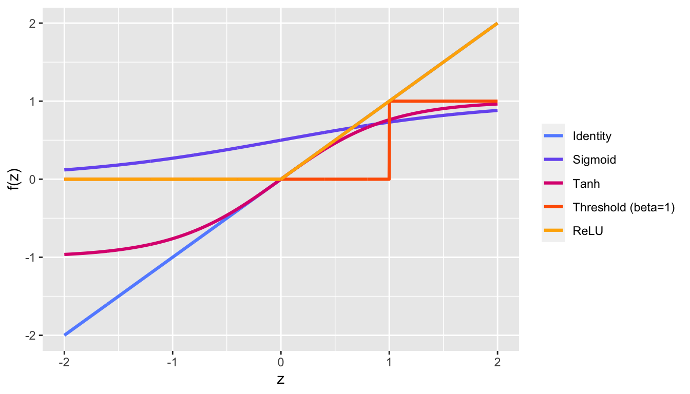
The activation function is the same for all units in a given layer. Once again, in the last layer, the choice of the activation function depends on the domain of the variable to predict and the number of units depends on the type of the data.
While Hornik, Stinchcombe, and White (1989) has shown that a feed-forward 3-layers (only one hidden) Neural Network with a finite number of neurons, with the same activation for each neuron in the hidden layer and the identity activation function for the output layer can approximate any bounded and regular function from \(\mathbb{R}^p\) to \(\mathbb{R}\). This universal approximation theorem therefore states that simple neural networks can represent a wide variety of functions. But, as stated by Goodfellow et al. (2016) :
“we are not guaranteed that the training algorithm will be able to learn that function.”
The optimisation algorithm may not be able to find the value of the parameters that corresponds to the desired function. Besides, there is a risk of overfitting:
“the layer may be infeasibly large and may fail to learn and generalize correctly”
Adding more hidden layers with a modest number of neurons in each should make the learning task easier, as stated in James et al. (2021).
We can illustrate how a multilayer perceptron works by being original (or not) and by taking the example of the famous MNIST dataset (Modified National Institute of Standards) database (Lecun et al. 1998). It contains a training set of 60,000 examples of handwritten digits (0 to 9) and a test set of 10,000 examples. In this database, the digits have been size-normalized and centered to fit into a \(28\times 28\) pixel bounding box. Each pixel of each \(28\times 28\) image have a grayscale value in the range \(0:255\).
The data can be accessed through the package {keras}. Keras is a deep learning framework which allows us to build and train deep-learning models. We will use the R interface to Keras (https://keras.rstudio.com/). To be able to use Keras, not only do we need to install the {keras} package, but we also need to install a backend tensor engine. We can, for instance, install TensorFlow.
We can first install the {tensorflow} package:
install.packages("tensorflow")Then the {keras} package:
install.packages("keras")Once the package is installed, it can be loaded.
library(keras)Then, TensorFlow can be installed:
tensorflow::install_tensorflow()And can be configured:
tensorflow::tf_config()Then, we need to install the core Keras library (we only do it once). If no python environment is found, we may agree to install Miniconda.
install_keras()On one of my computers running on MacOS Big Sur version 11.6, with R 4.0.5, I had an error during the installation (“error code 1”). I used the following instructions to solve the problem:
unlink(reticulate::miniconda_path(), recursive = TRUE)
reticulate::install_miniconda(path = reticulate::miniconda_path(),
                              update = TRUE, force = FALSE)
keras::install_keras()
If our computer is equipped with an NVIDIA GPU (Graphics Processing Unit) and our system configured with CUDA and cuDNN libraries, we can install the GPU-based version of the backend engine. Otherwise, we can stick with the CPU-based (Central Processing Unit) version. The installation needs to be done only once.
# install_keras(tensorflow = "gpu")Let us load the MNIST dataset:
mnist <- dataset_mnist()It is a list of two arguments: the train set, and the test set. The train set contains \(n=60,000\) images (observations/training examples). They are stored as an array. Recall that each image is made of 28x28 pixels. Hence, each example has \(p=28\times28=784\) predictors/features.
x_train <- mnist$train$x
dim(x_train)
## [1] 60000 28 28There are \(10,000\) observations in the test set:
x_test <- mnist$test$x
dim(x_test)
## [1] 10000 28 28The corresponding labels (true values), \(y\):
y_train <- mnist$train$y
head(y_train)
## [1] 5 0 4 1 9 2And for the test set:
y_test <- mnist$test$y
head(y_test)
## [1] 7 2 1 0 4 1Another way to assign the content of the elements of the list mnist to the four objects (x_train, y_train, x_test, and y_test) is to use the multi-assignment operator %<-% from {zeallot} (the operator is available if {keras} is loaded).
c(c(x_train, y_train), c(x_test, y_test)) %<-% mnistThere is approximatively 10% of each of the 10 different classes (0, 1, 2, …, 9):
round(100*prop.table(table(y_train)),1)## y_train
## 0 1 2 3 4 5 6 7 8 9
## 9.9 11.2 9.9 10.2 9.7 9.0 9.9 10.4 9.8 9.9We can visualize on a graph how the first example looks like. It is labelled as 5:
y_train[1]## [1] 5Let us create a function to change a training example with its 784 characteristics back to a matrix of 28x28 pixels, and then, let us define another small function to plot this matrix.
rotate <- function(x) t(apply(x, 2, rev))
convert_example_tibble <- function(example){
    rotate(example) %>%
    reshape2::melt(c("xx", "yy"),
                 value.name = "grey_scale") %>%
  as_tibble()
}

plot_example <- function(example){
  ggplot(data = convert_example_tibble(example),
       mapping = aes(x = xx, y = yy, fill = grey_scale))+
  geom_tile() +
  coord_equal() +
  scale_fill_gradient("Grey Scale", low = "white", high = "black")
}plot_example(x_train[1,,])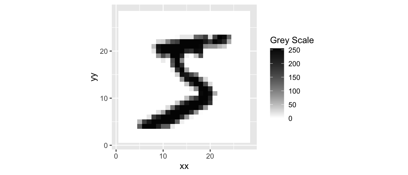
Figure 6.3: The first observation in the training set is a 5.
The first 10 observations from MNIST training set :
map_df(1:10, ~convert_example_tibble(x_train[.,,]), .id = "ind") %>%
  mutate(ind = as.numeric(ind)) %>%
  left_join(tibble(y = y_train[1:10], ind = 1:10),
            by = "ind") %>%
  mutate(lab = str_c("ex. ", ind, ": ", y)) %>%
  ggplot(data = .,
       mapping = aes(x = xx, y = yy, fill = grey_scale))+
  geom_tile() +
  coord_equal() +
  scale_fill_gradient("Grey Scale", low = "white", high = "black") +
  facet_wrap(~lab, ncol = 5) +
  theme(axis.text = element_blank(), axis.ticks = element_blank()) +
  labs(x = NULL, y = NULL)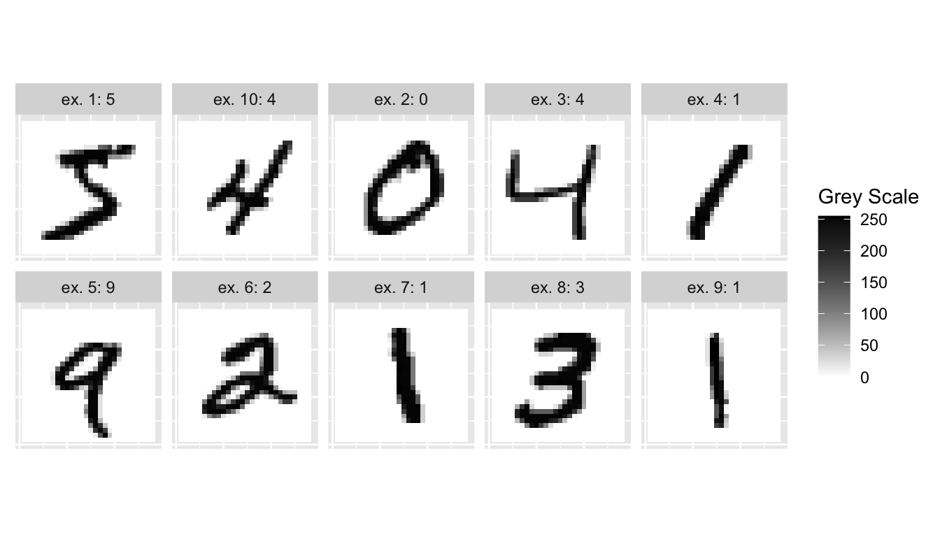
Figure 6.4: The first 10 observations from the MNIST dataset.
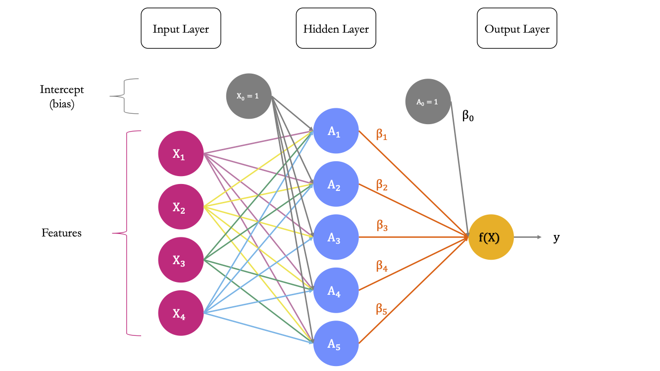
Figure 6.5 shows a diagram explaining the architecture of a multilayer perceptron suitable to classify the observations from the MNIST dataset. It has two hidden layers.
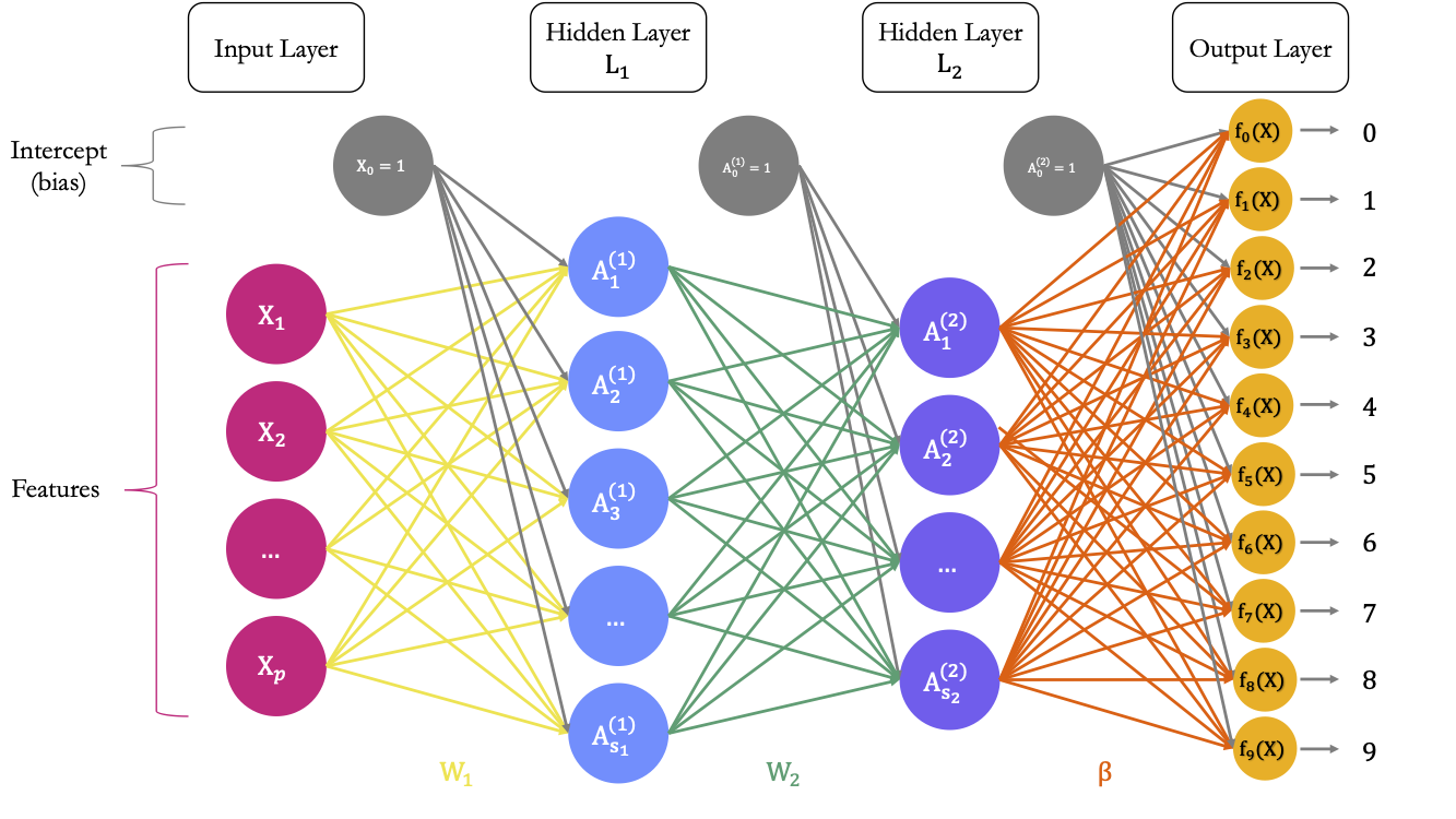
Figure 6.5: A Neural Network with \(p\) predictors, two hidden layer, and 10 outputs.
Input Layer
The first layer is the input layer. It contains 784 neurons (\(p=784\) pixels for an observation.
Output Layer
The last layer is the output layer. As we wish to build a classifier for \(M=10\) classes, the last output needs to contain M = 10 units. In a first step, 10 different models will be constructed, using a linear combination of the input provided by the previous layer, i.e., the \(\color{IBMPurple}{S_2}\) values and an intercept. Hence, for model \(m\), with \(m=0,1,\ldots,9\)
\[\begin{align} \color{IBMYellow}{Z_m} & = \color{gray}{\beta_{0,m}}\color{black} + \sum_{s=1}^{\color{IBMPurple}{S_2}}\color{black} \color{wongOrange}{\beta_{s,m}}\color{IBMPurple}{h_s^{(2)}}\color{black}(\mathbf{\color{IBMPurple}x\color{black}})\\ & = \color{gray}{\beta_{0,m}}\color{black} + \sum_{s=1}^{\color{IBMPurple}{S_2}}\color{black} \color{wongOrange}{\beta_{s, m}}\color{IBMPurple}{A_{s}^{(2)}} \end{align}\]
Each unit receives the output of the previous layer as an input as well as an intercept. It computes a linear combination of these outputs of the previous layer and this intercept. In total, there are \((S_2+1)\times M\) weights to estimate in the matrix \(\color{wongOrange}{\beta}\) of weights.
Then, in a second step, an activation function can be applied. Here, as we wish to obtain probabilities associated to each of the classes (0, 1, … 9), the activation function is not applied to each unit separately. We would like each unit to return the probability that an observation is of class \(m\), i.e., for \(m=0,1, \ldots,9)\), we would like to obtain:
\[\begin{align} \color{IBMYellow}{f_m}\color{black}(\color{IBMMagenta}{\mathbf{x}}\color{black}) = \mathbb{P}\left( y = m \vert \color{IBMMagenta}{\mathbf{x}}\color{black}\right). \end{align}\]
A way to do so is to use a softmax activation function: \[\begin{align} \color{IBMYellow}{f_m}\color{black}(\color{IBMMagenta}{\mathbf{x}}\color{black}) = \frac{\exp({\color{IBMYellow}{Z_m}\color{black}})}{\sum_{s=0}^{9} \exp(\color{IBMYellow}{Z_s}\color{black})}. \end{align}\]
6.1.2.1 Practice With Keras: classifier
Let us use Keras to create the architecture. We will use the keras_model_sequential() function to create a linear stack of layers. Our neural network will be made of two hidden layers with \(S_1 = 256\) and \(S_2 = 128\) units in the first and in the second layers, respectively. These layers will be densely connected (or, fully connected): each output from the previous layer is connected to each input in the current layer. To create a layer, we can use the layer_dense() function. The number of units in a later are specified with the units argument, while the activation function is specified using the activation argument (if no activation is specified, the identity function is applied).
Recall that each observation/training example is, in our case, a \(28\times 28\) matrix, stored in an array. We will use the array_reshape() function from {reticulate} to reshape the observation to obtain a matrix with each row corresponding to an observation and each column to a predictor.
x_train <- array_reshape(x_train, dim = c(nrow(x_train), 784))
x_test <- array_reshape(x_test, dim = c(nrow(x_test), 784))
Before feeding the data to the model, we need to preprocess it so that the values are scaled down to \([0,1]\). This helps the algorithm to converge to a solution. (The weights used are randomly chosen with small values at the beginning of the optimisation iterative process. Scaling the input – and output if it is a numeric variable – will reduce the problem complexity of the problem that the neural network tries to solve). Here, as the pixels correspond to grayscale intensity (0: black, 255:white), we can simply divide the values by the maximum and will get values between 0 and 1.
x_train <- x_train/255The response variable is for now numerical. Let us transform it to a qualitative (factor) variable. Since the target has 10 classes, we will get a matrix with 10 columns, each containing a dummy variable. We thus convert a vector of integers to a binary class matrix. This process is referred to as one-hot encoding.
y_train <- to_categorical(y_train)We also need to apply the same transformation to the test set:
x_test <- x_test/255
y_test <- to_categorical(y_test)
Lastly, just before we set up the architecture of the model, let us set some observations aside to observe the performances of the model during the iterative training process. The model will train on some data (train set), we will monitor its performances on unseen data (validation set). We do this, because if we change the structure of the model, we need to be able to know which model performs best. The test data will then be used to know how the “best” model may perform when used on entirely new data. In a way, the data in the validation set may not serve to train the model, but they are used to fine tune it. They are thus not entirely unseen.
n_valid <- round(.2*nrow(x_train))
ind_partial_valid <-
  sample(1:nrow(x_train), size = n_valid, replace =  FALSE)

x_train_partial <- x_train[-ind_partial_valid, ]
x_validation <- x_train[ind_partial_valid, ]

y_train_partial <- y_train[-ind_partial_valid,]
y_validation <- y_train[ind_partial_valid,]dim(x_train_partial)## [1] 48000 784dim(x_validation)## [1] 12000 784dim(y_train_partial)## [1] 48000 10dim(y_validation)## [1] 12000 10Here is our sequential model:
model_architecture <-
  keras_model_sequential(name = "MNIST_Model") %>%
  # First hidden layer
  layer_dense(units = 256, activation = "relu",
              input_shape = 784) %>%
  # Second hidden layer
  layer_dense(units = 128, activation = "relu") %>%
  # Output layer
  layer_dense(units = 10, activation = 'softmax')
Let us have a look at the informations provided:
model_architecture## Model
## Model: "MNIST_Model"
## ________________________________________________________________________________
## Layer (type) Output Shape Param #
## ================================================================================
## dense_2 (Dense) (None, 256) 200960
##
## dense_1 (Dense) (None, 128) 32896
##
## dense (Dense) (None, 10) 1290
##
## ================================================================================
## Total params: 235,146
## Trainable params: 235,146
## Non-trainable params: 0
## ________________________________________________________________________________The first layer is the input data: there is 60,000 training examples, but we have not yet fed them to the model. In the first hidden layer (dense_2) \(L_1\), the number of parameters to estimate is \((784+1) \times 256= 200,960\). In the second hidden layer (dense_1) \(L2\), the number of parameters to estimate is \((256+1) \times 128 = 32,896\). In the output layer (dense), the number of parameters to estimate is \((128+1)\times 10 = 1,290\).
Once the architecture of the model is set, we still need to decide:
- which objective function to use (which loss function)
- which optimizer to use
- which metrics to evaluate during training and testing.
These three aspects are set through the compile() from {generics}. Let us use the following:
loss: since we want to build a classifier (the response variable/target is qualitative), we can use the cross entropy (the model will seek to minimise the negative multinomial log-likelihood)
\[-\sum_{i=1}^{60,000} \sum_{m=0}^{9} = y_{i,m} \log(f_m(x_i))\]
optimizer: we will use the default optimizer, called “rmsprop,” which is an extension of gradient descent
- if we want to specifically set the learning rate and the decay to values, let us say 0.01 and \(10^-6\), respectively, we can set the optimizer to :
optimizer_rmsprop(lr=0.01, decay = 1e-6)metrics: the model will evaluate the accuracy through the iterations.
Let us do it (the changes are made in-place, we do not make a new assignment with <-):
model_architecture %>%
  compile(
    loss = "categorical_crossentropy",
    optimizer = "rmsprop",
    metrics = c("accuracy")
  )
It is possible to use a user-defined loss function, and/or metrics.
To define a custom metric function, it is possible to use the custom_metric() function from {keras}. The syntax is the following:
custom_metric(name, metric_fn)where name is the desired name of the metric (a string), and metric_fn is a function with the following signature function(y_true, y_pred), that accepts tensors.
However, there is a high chance that the metric we want to use has already been coded (mean squarred error, accuracy, auc, crossentropy, cosine similarity, …)
To get the list of all the ready-to-use loss functions, we can type ?loss-functions in the console.
Now that we are all set, the neural network can be trained, using the fit() function. We can specify the number of epochs (we will only use 10 here) as well as the size of the batches (we will set it to 128). Recall from the first hands-on session that increasing the size of the batches leads to less noisy optimisation process (but fasten the computation). During the training, it is possible to follow the loss and the desired metrics on the validation sample: we just need to provide the validation set through a list to the validation_data argument.
mnist_model_hist <-
  model_architecture %>%
  fit(x_train_partial, y_train_partial,
      epochs = 20, batch_size = 128,
      validation_data = list(x_validation, y_validation))
During the training, after each epoch, the loss function is evaluated and the result is printed in the console as well as plotted on a graph to monitor the process. As we also asked the accuracy to be reported, it is computed after each epoch and reported both on the console and on a graph too.
We assigned the output returned by fit() to an object we named mnist_model_hist. This way, we can access the different metrics computed during the training process.
mnist_model_hist$metrics## $loss
## [1] 0.294749498 0.115315005 0.076535478 0.054404959 0.041911248 0.031840410
## [7] 0.024246907 0.018707141 0.015080354 0.012119832 0.009452516 0.007689864
## [13] 0.006182983 0.005007274 0.005078920 0.004429060 0.003973258 0.003519077
## [19] 0.002576303 0.002296944
##
## $accuracy
## [1] 0.9130625 0.9658750 0.9762292 0.9831458 0.9873750 0.9902500 0.9926667
## [8] 0.9942709 0.9952708 0.9961458 0.9968750 0.9974583 0.9978750 0.9983959
## [15] 0.9984583 0.9986042 0.9988125 0.9987292 0.9991041 0.9991875
##
## $val_loss
## [1] 0.15497054 0.11522171 0.08932213 0.09704802 0.09755370 0.10156651
## [7] 0.08734521 0.08598512 0.09692394 0.09851355 0.12780029 0.11920659
## [13] 0.12321968 0.14193113 0.13232668 0.14073463 0.13415202 0.14239880
## [19] 0.16715638 0.16219296
##
## $val_accuracy
## [1] 0.9535000 0.9659167 0.9726667 0.9704167 0.9716667 0.9729167 0.9765834
## [8] 0.9760000 0.9762500 0.9773333 0.9742500 0.9760833 0.9780833 0.9743333
## [15] 0.9771667 0.9757500 0.9780000 0.9778333 0.9756666 0.9775000plot(mnist_model_hist)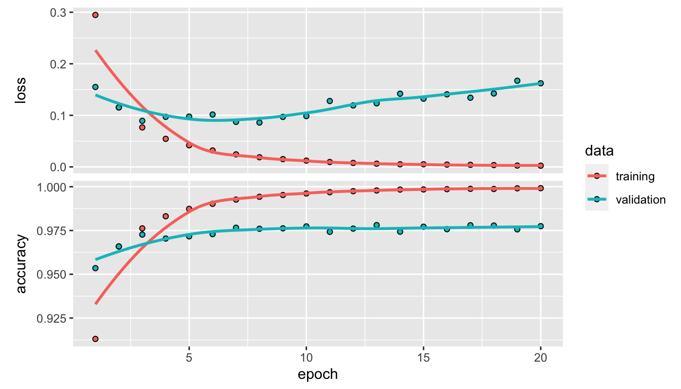
Figure 6.6: Accuracy and loss after each epoch, both on the training and validation sets.
Just for fun, we can also create our own graph:
as_tibble(mnist_model_hist$metrics) %>%
  mutate(epoch = row_number()) %>%
  pivot_longer(cols = -epoch) %>%
  mutate(data = ifelse(str_detect(name, "^val_"), "validation", "training"),
         name = str_remove(name, "^val_")) %>%
  ggplot(data = .,
         mapping = aes(x = epoch, y = value, colour = data)) +
  geom_line() +
  geom_point() +
  scale_colour_manual("Sample",
                      values = c("validation" = "#E69F00",
                                 "training" = "#0072B2")) +
  facet_wrap(~name, scales = "free_y", ncol = 1)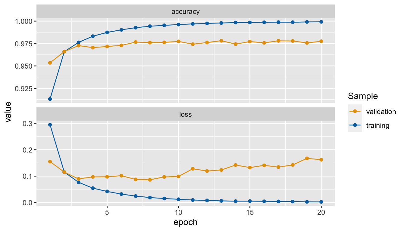
Figure 6.7: Accuracy and loss after each epoch, custom made graph.
We reached an accuracy 99.92%.
We notice that after the third epoch, the accuracy in the training set becomes higher than that of the validation set: we therefore face overfitting. We could then stop the training earlier to avoid overfitting and still have fair predictive capacities.
Let us have a look at the performances of the model on the test set. To do so, we can use the evaluate() function.
performances_test <- model_architecture %>%
  evaluate(x_test, y_test)
performances_test
## loss accuracy
## 0.149107 0.979500The accuracy in the test set is 97.95%.
To use the estimated model to make predictions, the function predict() can be used.
mnist_pred_test <- model_architecture %>% predict(x_test)As we have a multi-class target variable (10 classes), the model returned probabilities of belonging to each class. Hence, when we applied the predict() function on the test sample with \(10,000\) observations, we obtain a matrix with \(10,000\) rows and \(10\) columns.
For the first observation from the test sample, the predicted probabilities are the following:
mnist_pred_test[1,]## [1] 5.216950e-22 5.249442e-25 1.699038e-18 6.831150e-16 2.110166e-27
## [6] 5.990859e-20 3.190818e-32 1.000000e+00 1.109502e-25 7.978255e-18While the observed value is:
y_test[1, ]## [1] 0 0 0 0 0 0 0 1 0 0The first observation from the test set, if we predict the class based on the highest estimated probability is correctly predicted by the model.
We can make sure that the sum of the predicted probabilities, thanks to the softmax function used in the output layer, sum up to 1.
sum(mnist_pred_test[1,])## [1] 1Let us have a look at the predictive capacities for each categories. To do so, we first need to obtain the predicted class for each observation. We will predict the class of an observation based on the highest probability estimated by the model among the k classes.
mnist_pred_test_class <-
  as_tibble(mnist_pred_test, .name_repair = "unique") %>%
  mutate(pred_class = max.col(.),
         pred_class = seq(0,9)[pred_class]) %>%
  magrittr::extract2("pred_class")
The observed class:
mnist_test_class <-
  y_test %>%
  as_tibble(.name_repair = "unique") %>%
  mutate(y_class = max.col(.),
         y_class = seq(0,9)[y_class]) %>%
  magrittr::extract2("y_class")
The confusion table writes:
table(observed = mnist_test_class,
      predicted = mnist_pred_test_class)
## predicted
## observed 0 1 2 3 4 5 6 7 8 9
## 0 974 0 0 2 0 0 1 1 2 0
## 1 0 1128 1 1 0 0 2 1 2 0
## 2 4 8 995 4 2 0 2 8 9 0
## 3 0 0 5 983 0 8 1 5 2 6
## 4 2 0 2 0 964 0 3 3 1 7
## 5 2 0 0 6 3 872 4 1 3 1
## 6 4 3 1 1 9 2 936 0 2 0
## 7 0 6 5 1 1 0 0 1011 1 3
## [ getOption("max.print") est atteint -- 2 lignes omises ]A graph showing the percentage of correct predictions can be made. To that end, let us obtain the percentage of correct predictions for each class.
table_pct_pred <-
  tibble(
  observed = factor(mnist_test_class, levels = 0:9),
  predicted = factor(mnist_pred_test_class, levels = 0:9)
) %>%
  group_by(observed) %>%
  mutate(n_k = sum(n())) %>%
  group_by(observed, predicted, n_k) %>%
  count() %>%
  mutate(pred_pct = n / n_k) %>%
  ungroup() %>%
  select(observed, predicted, pred_pct)
table_pct_pred
## # A tibble: 73 × 3
## observed predicted pred_pct
## <fct> <fct> <dbl>
## 1 0 0 0.994
## 2 0 3 0.00204
## 3 0 6 0.00102
## 4 0 7 0.00102
## 5 0 8 0.00204
## 6 1 1 0.994
## 7 1 2 0.000881
## 8 1 3 0.000881
## 9 1 6 0.00176
## 10 1 7 0.000881
## # … with 63 more rowsIf we use this table directly, there will be missing cases. Let us complete it with 0 values when there are 0 predictions made for a given class when the true class is of class \(k\).
classes_mnist <-
  levels(factor(mnist_test_class, levels = 0:9))
df_plot_pred_mnist <-
  expand_grid(
  observed = classes_mnist,
  predicted = classes_mnist) %>%
  left_join(
    table_pct_pred
  ) %>%
  mutate(pred_pct = replace_na(pred_pct, 0))
The graph showing the percentage of predicted classes for each observed class can then be plotted.
ggplot(data = df_plot_pred_mnist,
       mapping = aes(x = predicted, y = observed,
                     fill = pred_pct,
                     label = round(pred_pct, 2))) +
  geom_tile() +
  geom_text(color = "white") +
  scale_fill_gradient("% of\n correct pred.",
                      low = "#1E88E5", high = "#D81B60") +
  labs(x = "Predicted", y = "Observed") +
  theme(panel.background = element_blank())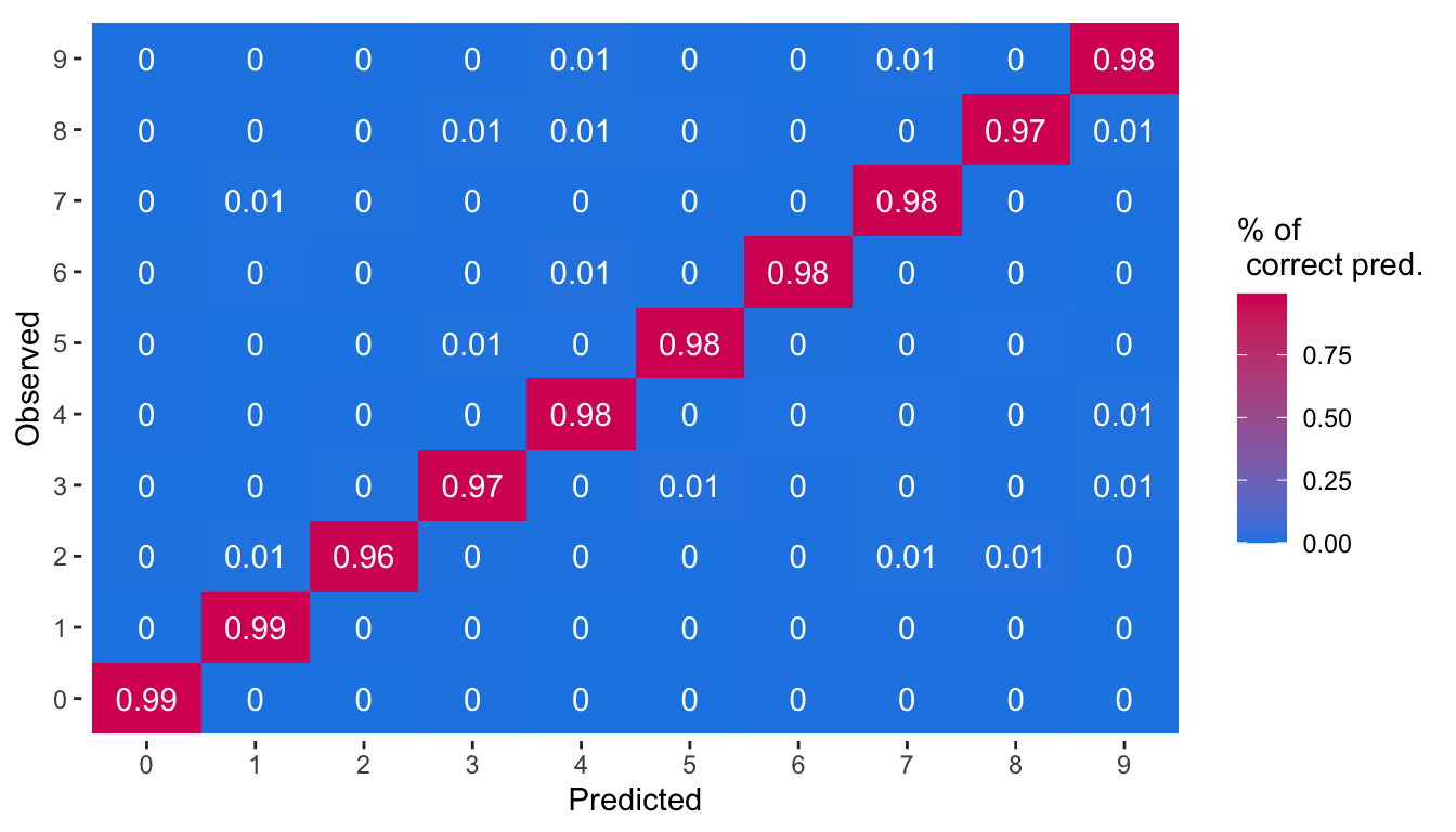
Figure 6.8: Percentage of predicted classes for each observed class.
Another way of looking at the predictive capacities consists in looking at the percentage of correctly predicted observation per class.
table_pct_pred_2 <-
  tibble(
  observed = factor(mnist_test_class, levels = 0:9),
  predicted = factor(mnist_pred_test_class, levels = 0:9)
) %>%
  mutate(correct = observed == predicted) %>%
  group_by(observed) %>%
  summarise(pct_correct = sum(correct) / n()) %>%
  mutate(pct_incorrect = 1-pct_correct) %>%
  pivot_longer(cols = -observed) %>%
  mutate(name = factor(name,
                       levels = c("pct_correct", "pct_incorrect"),
                       labels = c("Correctly predicted",
                                  "Incorrect predicted")))
The following graph can then be plotted.
ggplot(data = table_pct_pred_2,
       mapping = aes(x = name, y = observed,
                     fill = value,
                     label = round(value, 2))) +
  geom_tile() +
  geom_text(color = "white") +
  scale_fill_gradient("% of\n correct pred.",
                      low = "#1E88E5", high = "#D81B60") +
  labs(x = "Accuracy of prediction", y = "Observed") +
  theme(panel.background = element_blank())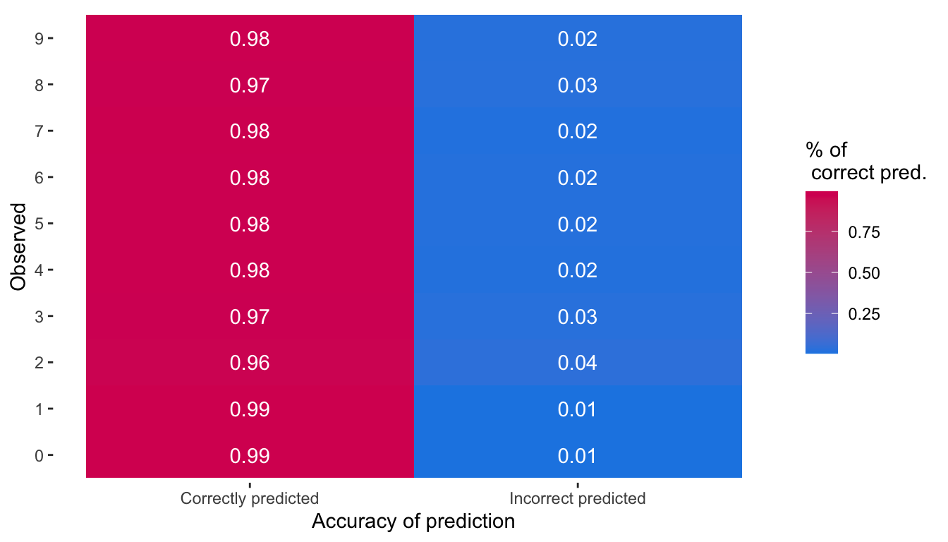
Figure 6.9: Percentage of correctly or incorrectly predicted observations by observed class.
The output layer is made of 10 units. Let us have a look at what happens if we just change one thing : the number of units in one of the hidden layers, such that it becomes very small compared to the number of classes to be predicted. We will here set the number of units in the second layer to only 2.
model_architecture_2 <-
  keras_model_sequential(name = "MNIST_Model_2") %>%
  # First hidden layer
  layer_dense(units = 256, activation = "relu",
              input_shape = 784) %>%
  # Second hidden layer
  layer_dense(units = 2, activation = "relu") %>%
  # Output layer
  layer_dense(units = 10, activation = 'softmax')
This is the only change. We will use the same optimizer and the same loss function.
model_architecture_2 %>%
  compile(
    loss = "categorical_crossentropy",
    optimizer = "rmsprop",
    metrics = c("accuracy")
  )
Let us train the model over 20 epochs and a batch size of 128, as earlier.
mnist_model_2_hist <-
  model_architecture_2 %>%
  fit(x_train_partial, y_train_partial,
      epochs = 20, batch_size = 128,
      validation_data = list(x_validation, y_validation))
mnist_model_2_hist
We clearly note that the accuracy of the model dropped. This is because the information was too compressed when going through the second layer.
as_tibble(mnist_model_hist$metrics) %>%
  mutate(model = "Initial model",
         epoch = row_number()) %>%
  bind_rows(as_tibble(mnist_model_2_hist$metrics) %>%
              mutate(model = "Second model",
                     epoch = row_number())) %>%
  pivot_longer(cols = -c(epoch, model)) %>%
  mutate(data = ifelse(str_detect(name, "^val_"),
                       "validation", "training"),
         name = str_remove(name, "^val_")) %>%
  ggplot(data = .,
         mapping = aes(x = epoch, y = value, colour = data,
                       linetype = model)) +
  geom_line() +
  geom_point() +
  scale_colour_manual("Sample",
                      values = c("validation" = "#E69F00",
                                 "training" = "#0072B2")) +
  facet_wrap(~name, scales = "free_y", ncol = 1) +
  labs(y = NULL)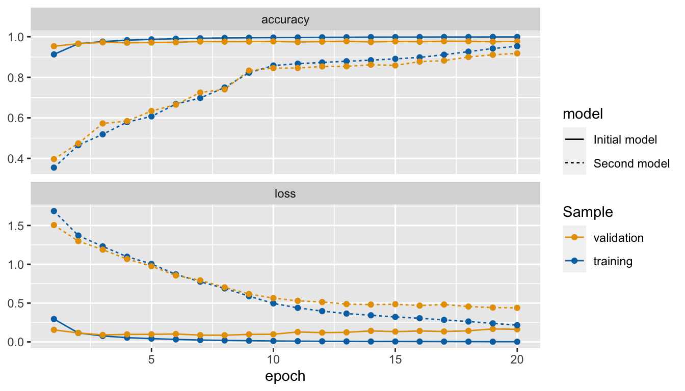
Figure 6.10: Accuracy and loss after each epoch, custom made graph.
To save the model using HDF5 files, {keras} provides the function save_model_hdf5().
if(!dir.exists("deep_learning_models"))
  dir.create("deep_learning_models")
model_architecture_2 %>%
  save_model_hdf5("deep_learning_models/mnist_model.h5")
A model saved in a HDF5 file can then be loaded using the load_model_hdf5() function:
model_architecture_2 <-
  load_model_hdf5("deep_learning_models/mnist_model.h5")
To destroy the current TensorFlow graph and create a new one, the function k_clear_session() can be used. This is useful to avoid clutter from previous models or layers.
k_clear_session()6.1.2.2 Practice With Keras: Regression
To illustrate how to build and estimate a neural network in a regression context, let us use the Seoul bike data from the second hands-on session.
load(url("http://egallic.fr/Enseignement/ML/ECB/data/bike.rda"))We have created new variable in the data during the second hands-on session. However, we still need to pre-process the data a little bit. While some functions such as lm(), svm() or glm() automatically create dummy variables in the design matrix whenever it contains a qualitative variable, this is not the case with the functions we use in {keras}. We thus need to manually transform categorical variables to dummy variables. We can use the dummy_cols() function from {fastDummies} to create dummy variables from character or factors. Here is a simple example:
library(fastDummies)
tibble(x = c("A", "B", "C"),
       y = factor(c("mon", "tue", "wed")),
       z = 1:3) %>%
  # Creating dummies for chr and fct
  dummy_cols(
    remove_first_dummy = TRUE,
    remove_selected_columns = TRUE)
## # A tibble: 3 × 5
## z x_B x_C y_tue y_wed
## <int> <int> <int> <int> <int>
## 1 1 0 0 0 0
## 2 2 1 0 1 0
## 3 3 0 1 0 1By setting remove_first_dummy = TRUE, we make sure to remove the first dummy of each categorical variable (to avoid colinearity), and by setting remove_selected_columns = TRUE we remove the original column from the table.
Let us do it with the bike dataset:
x_data <-
  bike %>%
  select(-date, -rented_bike_count, -y_binary) %>%
  dummy_cols(
    remove_first_dummy = TRUE,
    remove_selected_columns = TRUE)
The variable to predict (the target) is the number of bikes rented each hour:
y_data <- bike$rented_bike_countLet us create the training and the test sets. For the moment, let us ignore the fact that bicycle rental data can be regarded as time-series. We will discuss sequentiality in the data later.
n_train <- round(.8*nrow(x_data))
set.seed(123)
ind_train <- sample(1:nrow(x_data), size = n_train, replace = FALSE)
The train set:
x_train <- x_data[ind_train, ]
y_train <- y_data[ind_train]
dim(x_train)
## [1] 6772 31length(y_train)## [1] 6772And the test set:
x_test <- x_data[-ind_train, ]
y_test <- y_data[-ind_train]
dim(x_test)
## [1] 1693 31length(y_test)## [1] 1693Let us scale the data, by removing to each variable \(x_j\), \(j=1,\ldots,p\) its mean \(\overline{x}_j\) and by dividing the result by its standard deviation \(\sigma_{x_k}\): \(\frac{x_j - \overline{x}_j}{\sigma_{x_j}}\). We thus need to compute the mean and standard deviation of each variable in the training test:
mean_train <- apply(x_test, 2, mean)
std_train <- apply(x_test, 2, sd)
Then, the data from both the train and test set can be scaled:
x_train <- scale(x_train, center = mean_train, scale = std_train)
x_test <- scale(x_test, center = mean_train, scale = std_train)
Note that the data from the test set were scaled using the means and standard deviations computed on the train set.
Let us create a function that defines the model depending on the train data. As the number of observation is modest, we will only consider a small network with three hidden layers. We will monitor the Mean Absolute Error (MAE) :
\[\text{MAE} = \frac{1}{n} \sum_{i=1}^{n} \lvert y_i - \widehat{y}_i \rvert.\]
model_structure_bike <- function(train_data) {
  model <-
    keras_model_sequential() %>%
    # First hidden layer
    layer_dense(units = 128, activation = "relu",
                input_shape = dim(train_data)[[2]]) %>%
    # Second hidden layer
    layer_dense(units = 128, activation = "relu") %>%
    # Third hidden layer
    layer_dense(units = 64, activation = "relu") %>%
    # Output layer
    layer_dense(units = 1)

  model %>%
    compile(
    optimizer = "rmsprop",
    loss = "mse",
    metrics = c("mae")
) }
We will use 5-fold cross-validation to evaluate the neural network. We do so because we will need to adjust some parameters of the model to find one that suits us (we can change the number of hidden layers and their number of respective units, the number of epochs, the batch size, and so on). We therefore need to compare the models with each other.
nb_folds <- 5Here are the assignment of the folds:
set.seed(123)
folds <- sample(rep(1:nb_folds, length=nrow(x_train)))
Let us set the number of epoch to 10 and the batch size to 1. Recall from the first hands-on session that setting the batch size to 1 means that during an epoch, each observation will be used in turn to update the parameters of the models.
num_epochs <- 10
batch_size <- 32
loss_and_metrics <- NULLBy using verbose = 0 in the functions fit() and evaluate(), the model is trained silently, without either plotting the loss and MAE nor printing the values in the console.
for(k in 1:nb_folds){
  # cat(str_c("\nFold number: ", k, "\n"))

  ind_current <- folds != k

  # Train set
  x_train_partial <- x_train[which(ind_current),]
  y_train_partial <- y_train[which(ind_current)]

  # Validation set
  x_train_valid <- x_train[which(!ind_current),]
  y_train_valid <- y_train[which(!ind_current)]

  # Building the model
  model <- model_structure_bike(x_train_partial)

  # Training the model on the training set
  model %>%
    fit(x_train_partial, y_train_partial,
        epochs = num_epochs, batch_size = batch_size, verbose = 0)

  # Evaluating its performances on test data
  results_current <- model %>%
    evaluate(x_train_valid, y_train_valid, verbose = 0)

  # Store loss and metrics
  loss_and_metrics <-
    loss_and_metrics %>% bind_rows(
      as_tibble(t(results_current)) %>%
        mutate(fold = k)
    )
}
The computed metrics with thus version of the neural network:
loss_and_metrics## # A tibble: 5 × 3
## loss mae fold
## <dbl> <dbl> <int>
## 1 131442. 243. 1
## 2 140303. 255. 2
## 3 123807. 239. 3
## 4 119251. 234. 4
## 5 120723. 243. 5The average of the the Mean Average Error over the folds is:
mean(loss_and_metrics$mae)## [1] 242.6967That means that on average, our predictions are off by NA bikes. This is quite high, when compared to the distribution of the target variable.
summary(y_train)## Min. 1st Qu. Median Mean 3rd Qu. Max.
## 2.0 214.0 539.5 730.0 1087.0 3556.0Let us train the model over more epochs to see if it yields better results. Let us train it over 50 epochs.
num_epochs <- 800
batch_size <- 32
loss_and_metrics_2 <- vector(mode = "list", length = nb_folds)Warning: the following code takes about 15 minutes to run on a standard computer.
This time, let us keep track of the training history as in the first example with the MNIST dataset.
library(tictoc)

results <- vector(mode = "list", length = nb_folds)

tic()
for(k in 1:nb_folds){
  cat(str_c("\nFold number: ", k, "\n"))

  ind_current <- folds != k

  # Train set
  x_train_partial <- x_train[which(ind_current),]
  y_train_partial <- y_train[which(ind_current)]

  # Validation set
  x_train_valid <- x_train[which(!ind_current),]
  y_train_valid <- y_train[which(!ind_current)]

  # Building the model
  model <- model_structure_bike(x_train_partial)

  # Training the model on the training set
  history <-
    model %>%
    fit(x_train_partial, y_train_partial,
        validation_data = list(x_train_valid, y_train_valid),
        epochs = num_epochs, batch_size = batch_size, verbose = 0)

  # Evaluating its performances on test data
  results_current <- model %>%
    evaluate(x_train_valid, y_train_valid, verbose = 0)

    results[[k]] <- results_current

  # Store loss and metrics
  loss_and_metrics_2[[k]] <- history
}
toc()
Let us compute, for each epoch, the average of the 5-folds MAE both on the train and on the validation samples:
mae_mean_folds <-
  map(loss_and_metrics_2, "metrics") %>%
  map("val_mae") %>%
  map_df(~as_tibble(.) %>% mutate(epoch = row_number()),
         .id = "fold") %>%
  mutate(sample = "validation") %>%
  bind_rows(
    map(loss_and_metrics_2, "metrics") %>%
      map("mae") %>%
      map_df(~as_tibble(.) %>% mutate(epoch = row_number()),
             .id = "fold") %>%
      mutate(sample = "train")
  ) %>%
  group_by(epoch, sample) %>%
  summarise(mae = mean(value), .groups = "drop")
mae_mean_folds
## # A tibble: 1,600 × 3
## epoch sample mae
## <int> <chr> <dbl>
## 1 1 train 440.
## 2 1 validation 300.
## 3 2 train 281.
## 4 2 validation 269.
## 5 3 train 263.
## 6 3 validation 264.
## 7 4 train 255.
## 8 4 validation 255.
## 9 5 train 250.
## 10 5 validation 258.
## # … with 1,590 more rowsLet us have a look at the metrics over the epochs:
ggplot(data = mae_mean_folds,
       mapping = aes(x = epoch, y = mae, colour = sample)) +
  geom_line() +
  scale_colour_manual("Sample",
                      values = c("validation" = "#E69F00",
                                 "train" = "#0072B2")) +
  labs(x = "Epoch", y = "MAE (validation sample)")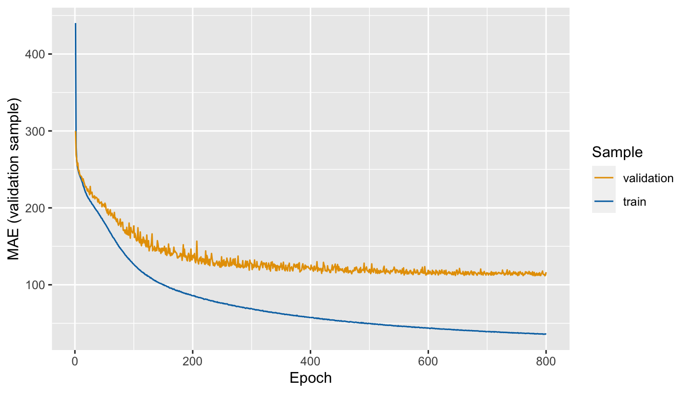
Figure 6.11: Mean Absolute Error (MAE) computed on the validation samples, over the epochs
The model overfits. The MAE seems to be stable after around 400 epochs. To avoid overfitting while keeping the number of observations constant, we can reduce both the number of layers and the number of units in them. We could also add weight regularization and add dropout. More on those aspects will be presented below.
Trying to adjust the model to find an architecture and hyperparameters that provides good results takes some time (this process is . It is possible to use a grid as in the second hands-on session to loop over different configurations of the network. After we have found a model that suits us, we can train a final one, which can then be used to make predictions on unseen data.
Warning: the following code takes about 5 minutes to run on a standard machine.
Let us say our final model is the following one:
num_epochs <- 400
batch_size <- 32
model <- model_structure_bike(x_train)
model %>%
    fit(x_train, y_train,
        epochs = num_epochs, batch_size = batch_size, verbose = 0)
When estimating the final model, we use the hyperparameters that lead to the best results, and we use the whole training dataset to train the algorithm.
The predictive abilities of the model on unseen data:
results_test <- model %>% evaluate(x_test, y_test)
results_test
## loss mae
## 31469.1484 105.77196.1.2.3 Regularisation techniques
6.1.2.3.1 Weight Regularization
Recall Emanuelle Flachaire’s course about penalised regressions such as Lasso, Ridge, or Elastic Net. In those regressions, the model is penalised for having too many variables. This is done through the introduction of a constraint in the model equation (and therefore in the loss function to be minimised).
The same idea of regularisation has been introduced in neural networks, to put some constraints on the complexity of the network, to avoid overfitting. These constraints are applied to the weights to force them to take only small values. Lasso (L1 norm) or Ridge (L2 norm/weight decay) regularisation on weights can be used.
Weight regularisation to the neural network with Keras is done by specifying the layer_dense() function with the argument kernel_regularizer. For example, for a L1 norm, we can use kernel_regularizer = regularizer_l1(l = 0.01), while for a L2 norm, we can use kernel_regularizer = regularizer_l2(l = 0.01).
To illustrate how regularisation techniques help to avoid overfitting, we will create a network that overfits. The risk of overfitting increases with the complexity of the model (controlled by the number of hidden layers and their respective number of units) and with the number of epochs the model is trained over.
Consider, again, the Seoul bike data. We will build a classifier to try to predict the binary variable y_binary that indicates whether the number of bikes rented per hours is belo 300 (“Low”) or not (“High”).
x_data <-
  bike %>%
  select(-date, -rented_bike_count, -y_binary) %>%
  dummy_cols(
    remove_first_dummy = TRUE,
    remove_selected_columns = TRUE)

# 1 if "Low", 0 otherwise
# y_data <- to_categorical(ifelse(bike$y_binary == "Low", yes = 1, no = 0))
y_data <- ifelse(bike$y_binary == "Low", yes = 1, no = 0)
The first 80% observations are kept for the train set and the remaining for the test set.
n_train <- round(.8*nrow(x_data))
set.seed(123)
ind_train <- sample(1:nrow(x_data), size = n_train, replace = FALSE)
The training test is thus:
x_train <- x_data[ind_train, ]
y_train <- y_data[ind_train]
dim(x_train)
## [1] 6772 31length(y_train)## [1] 6772And the test set:
x_test <- x_data[-ind_train, ]
y_test <- y_data[-ind_train]
dim(x_test)
## [1] 1693 31length(y_test)## [1] 1693The predictors can be scaled as previously, by demeaning with the values from the train set and dividing by the standard deviation, for each predictor.
mean_train <- apply(x_test, 2, mean)
std_train <- apply(x_test, 2, sd)
x_train <- scale(x_train, center = mean_train, scale = std_train)
x_test <- scale(x_test, center = mean_train, scale = std_train)
The predictive capacities of the model will be assessed on unseen data using 3-fold cross validation. The folds are assigned randomly:
nb_folds <- 3
set.seed(123)
folds <- sample(rep(1:nb_folds, length=nrow(x_train)))
Let us define a function constructing the architecture of the model, depending on the regularisation parameter of the L2 regularisation.
model_structure_bike_l2 <- function(train_data, l=0.01) {
  model <-
    keras_model_sequential() %>%
    # First hidden layer
    layer_dense(units = 32, activation = "relu",
                input_shape = dim(train_data)[[2]],
                kernel_regularizer = regularizer_l2(l)) %>%
    # Second hidden layer
    layer_dense(units = 64, activation = "relu",
                kernel_regularizer = regularizer_l2(l)) %>%
    # Third hidden layer
    layer_dense(units = 32, activation = "relu",
                kernel_regularizer = regularizer_l2(l)) %>%
    # Output layer
    layer_dense(units = 1, activation = "sigmoid")

  model %>%
    compile(
      optimizer = "rmsprop",
      loss = "binary_crossentropy",
      metrics = c("accuracy",
                  metric_true_positives(name = "tp"),
                  metric_true_negatives(name = "tn"),
                  metric_false_positives(name = "fp"),
                  metric_false_negatives(name = "fn"))
    )
}
Notice that the metrics argument of the compile() function takes a vector of arguments. Along with the accuracy, the number of true positives, true negatives, false positives, and false negatives will be reported, both for the train and the validation sets at each epoch, for each step of the k-fold cross-validation.
Let us train a model on 300 epochs, with a batch size of 512 observations.
num_epochs <- 300
batch_size <- 512

metrics_regul <-
  vector(mode = "list", length = nb_folds)

for(k in 1:nb_folds){
  cat(str_c("\nFold number: ", k, "\n"))

  ind_current <- folds != k

  # Train set
  x_train_partial <- x_train[which(ind_current),]
  y_train_partial <- y_train[which(ind_current)]

  # Validation set
  x_train_valid <- x_train[which(!ind_current),]
  y_train_valid <- y_train[which(!ind_current)]

  # Building the model
  model_with_regul <- model_structure_bike_l2(x_train_partial, l = 0.01)

  # Training the model on the training set
  history <-
    model_with_regul %>%
    fit(x_train_partial, y_train_partial,
        validation_data = list(x_train_valid, y_train_valid),
        epochs = num_epochs, batch_size = batch_size, verbose = 0)

  # Store loss and metrics
  metrics_regul[[k]] <- history
}
For comparison, a model without regularisation can be trained. First, a function that creates the architecture of the model can be defined.
model_structure_bike <- function(train_data) {
  model <-
    keras_model_sequential() %>%
    # First hidden layer
    layer_dense(units = 32, activation = "relu",
                input_shape = dim(train_data)[[2]]) %>%
    # Second hidden layer
    layer_dense(units = 64, activation = "relu") %>%
    # Third hidden layer
    layer_dense(units = 32, activation = "relu") %>%
    # Output layer
    layer_dense(units = 1, activation = "sigmoid")

  model %>%
    compile(
      optimizer = "rmsprop",
      loss = "binary_crossentropy",
      metrics = c("accuracy",
                  metric_true_positives(name = "tp"),
                  metric_true_negatives(name = "tn"),
                  metric_false_positives(name = "fp"),
                  metric_false_negatives(name = "fn"))
    )
}
Then, the predictive abilities of the model can be assessed on the validation sets during the 3-fold cross-validation.
num_epochs <- 500
batch_size <- 512

metrics_without_regul <-
  vector(mode = "list", length = nb_folds)


for(k in 1:nb_folds){
  cat(str_c("\nFold number: ", k, "\n"))

  ind_current <- folds != k

  # Train set
  x_train_partial <- x_train[which(ind_current),]
  y_train_partial <- y_train[which(ind_current)]

  # Validation set
  x_train_valid <- x_train[which(!ind_current),]
  y_train_valid <- y_train[which(!ind_current)]

  # Building the model
  model <- model_structure_bike(x_train_partial)

  # Training the model on the training set
  history <-
    model %>%
    fit(x_train_partial, y_train_partial,
        validation_data = list(x_train_valid, y_train_valid),
        epochs = num_epochs, batch_size = batch_size, verbose = 0)

  # Store loss and metrics
  metrics_without_regul[[k]] <- history
}
Let us define a function to extract the metric values from the history stored during the k-fold cross-validation process. This function will return the average over the k folds for each epoch, in a tibble.
#' @param k_fold_history list with the training history during the k-fold CV
#' @param metric (string) name of the metric to extract from the history
history_to_tibble <- function(k_fold_history, metric){
  map(k_fold_history, "metrics") %>%
    # Metrics on the validation sets
    map(str_c("val_",metric)) %>%
    map_df(~as_tibble(.) %>% mutate(epoch = row_number()),
           .id = "fold") %>%
    mutate(sample = "validation") %>%
    bind_rows(
      map(k_fold_history, "metrics") %>%
        map(metric) %>%
        map_df(~as_tibble(.) %>% mutate(epoch = row_number()),
               .id = "fold") %>%
        mutate(sample = "train")
    ) %>%
    group_by(epoch, sample) %>%
    summarise(!!sym(metric) := mean(value), .groups = "drop") %>%
    mutate(sample = factor(sample, levels = c("validation", "train")))
}
Let us apply this function to the list containing the history of the training without regulation, and then with a L2 regularization.
df_metrics_regul <-
  history_to_tibble(metrics_without_regul, "accuracy") %>%
  mutate(type = "Without regularisation") %>%
  bind_rows(
    history_to_tibble(metrics_regul, "accuracy") %>%
      mutate(type = "L2 regularisation (l=0.01)")
  )

df_metrics_regul
## # A tibble: 1,200 × 4
## epoch sample accuracy type
## <int> <fct> <dbl> <chr>
## 1 1 train 0.685 Without regularisation
## 2 1 validation 0.737 Without regularisation
## 3 2 train 0.769 Without regularisation
## 4 2 validation 0.789 Without regularisation
## 5 3 train 0.800 Without regularisation
## 6 3 validation 0.807 Without regularisation
## 7 4 train 0.814 Without regularisation
## 8 4 validation 0.816 Without regularisation
## 9 5 train 0.823 Without regularisation
## 10 5 validation 0.822 Without regularisation
## # … with 1,190 more rowsThen we can look at the results:
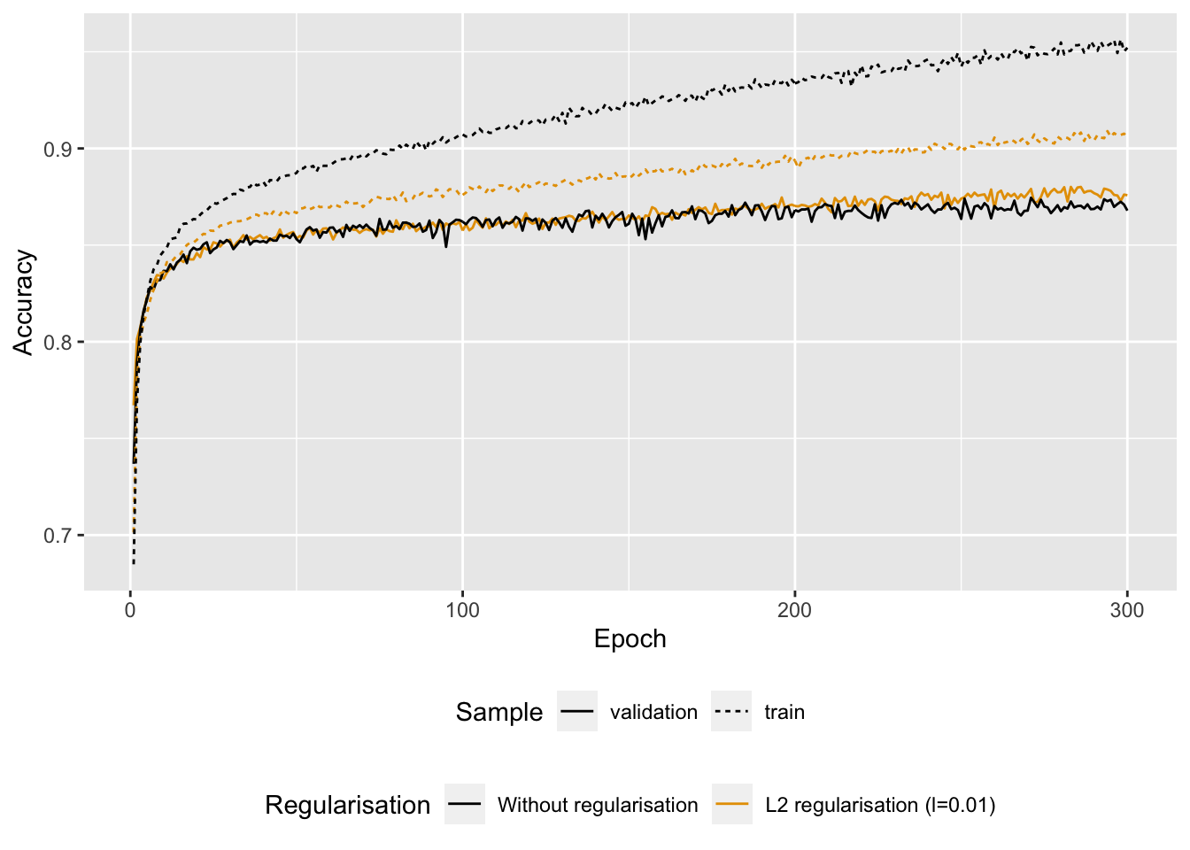
Figure 6.12: Accuracy with or without regularisation.
We note that the model with L2 regularisation is less prone to overfitting than the model where no penalisation on the weights was applied.
6.1.2.3.2 Dropout
Consider a layer with its \(S_1\) units: it outputs \(S_1\) values. When dropout is applied to a layer, some of its outputs are randomly set to 0: they are dropped out. During the training process, a fraction of the outputs of the layer to which dropout is applied are set to zero: this fraction is called the dropout rate.
This corresponds to assigning to each unit of the layer a probability of being dropped out, during each iterations of the training phase. Usually, the droupout rate rate of a hidden layer is set to 0.5.
During the test phase, none of the outputs of the units will be set to 0. Instead, the output of the layer, at the time of the test, is scaled to take into account that the outputs of some of the units have been randomly set to 0.
It is therefore a technique that adds noise, in order to prevent the model from learning certain particularities that are specific to the training data and that cannot then be generalised to the whole data set.
Let us look at a simple example with a small neural network with. Then, we can look at how to perform dropout in R.
Assume that we have only 4 explanatory variables, 2 hidden layers (the first one with 5 unites and the second with 4 unit), and that we want to predict a numerical output variable. Let us apply dropout regularisation only on the second hidden layer. The corresponding architecture of the network is depicted in Figure 6.13.
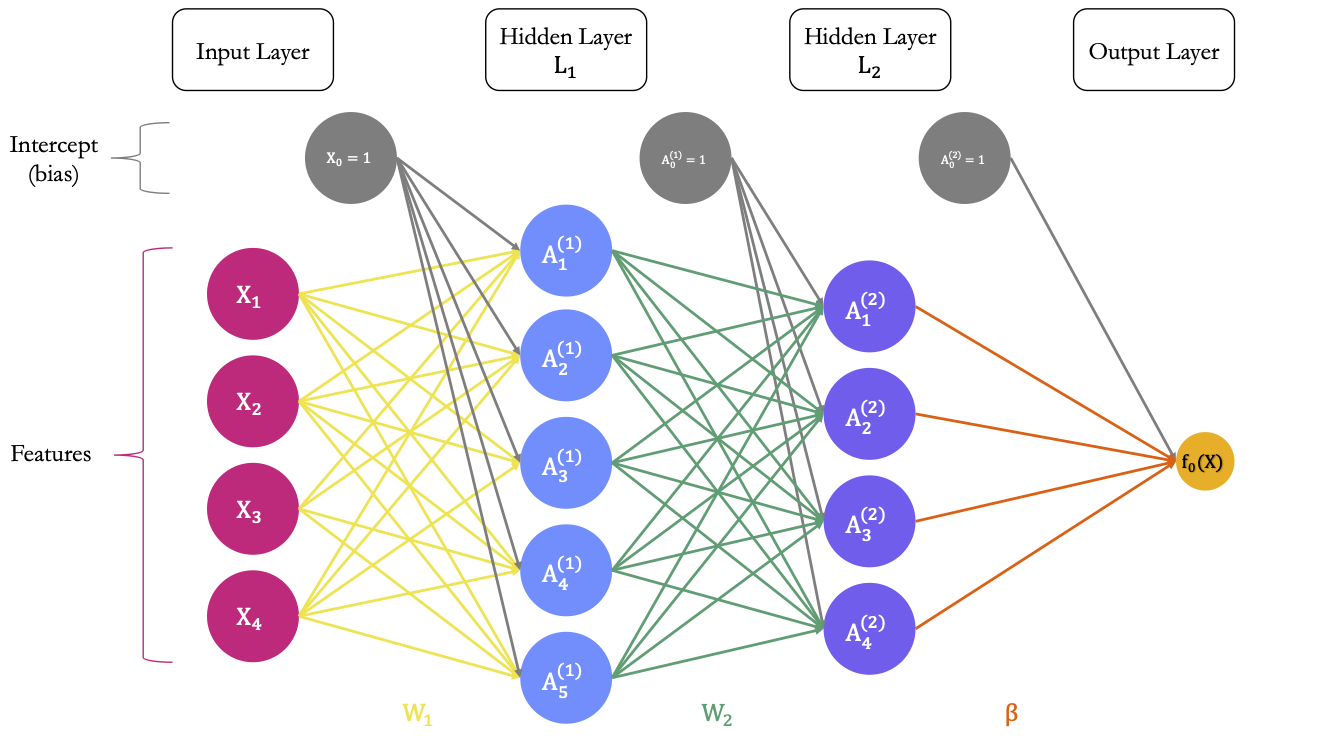
Figure 6.13: Estimated parameters of the model before applying the droupout.
Now, let us say that we apply dropout regularisation to the first and second hidden layers, using a dropout rate of .5. For each layer, on average, .5 of the units will be dropped out at each iteration. Assume that for our current example, the 2nd and 4th unit of the first hidden layer were randomly picked to be dropped out, as well as the first two units of the second hidden layer. The situation is illustrated in 6.14.
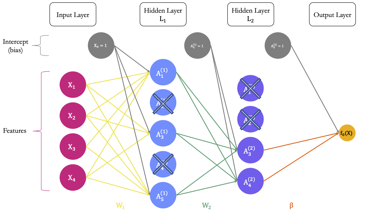
Figure 6.14: Dropout regularisation: each unit of the hidden layer has a probability to be dropped out.
One of the most used techniques to implement this dropout regularisation is called inverted dropout. Let us use some R codes to illustrate how it is applied. Let us define the weight matrices as well as the matrix of coefficients \(\beta\) (we assume the following values obtained from previous iteration of the backward propagation algorithm).
Let us simulate some data.
set.seed(123)
x <- rnorm(4)
Assume that our weight matrix \(W_1\) is:
W_1 <- matrix(round(rnorm(20), 2), ncol = 5)
colnames(W_1) <- str_c("L1 Unit ", 1:5)
W_1
## L1 Unit 1 L1 Unit 2 L1 Unit 3 L1 Unit 4 L1 Unit 5
## [1,] 0.13 -0.69 0.40 0.50 -1.07
## [2,] 1.72 -0.45 0.11 -1.97 -0.22
## [3,] 0.46 1.22 -0.56 0.70 -1.03
## [4,] -1.27 0.36 1.79 -0.47 -0.73The weight matrix \(W_2\):
W_2 <- matrix(round(rnorm(20), 2), ncol = 4)
colnames(W_2) <- str_c("L2 Unit ", 1:4)
W_2
## L2 Unit 1 L2 Unit 2 L2 Unit 3 L2 Unit 4
## [1,] -0.63 1.25 0.82 -0.38
## [2,] -1.69 0.43 0.69 -0.69
## [3,] 0.84 -0.30 0.55 -0.21
## [4,] 0.15 0.90 -0.06 -1.27
## [5,] -1.14 0.88 -0.31 2.17And the \(\beta\) matrix:
beta <- c(0.23, -0.10, 0.13, 0.02)Then the bias:
bias_0 <- rnorm(5)
bias_1 <- rnorm(4)
bias_2 <- rnorm(1)

bias_0
## [1] 1.2079620 -1.1231086 -0.4028848 -0.4666554 0.7799651bias_1## [1] -0.08336907 0.25331851 -0.02854676 -0.04287046bias_2## [1] 1.368602Each unit of the first hidden layer makes a linear combination of the inputs, using the current weights.
linear_comb_layer_1 <- x %*% W_1 + bias_0
linear_comb_layer_1
## L1 Unit 1 L1 Unit 2 L1 Unit 3 L1 Unit 4 L1 Unit 5
## [1,] 1.366655 1.294207 -1.399061 0.7645134 -0.2266276Then, let us say we use a ReLU function for the first hidden layer. The output value of each unit is then:
A_k_layer_1 <- relu_f(linear_comb_layer_1)
A_k_layer_1
## [1] 1.3666550 1.2942066 0.0000000 0.7645134 0.0000000The linear combination made in the second layer, by each unit:
linear_comb_layer_2 <- A_k_layer_1 %*% W_2 + bias_1
linear_comb_layer_2
## L2 Unit 1 L2 Unit 2 L2 Unit 3 L2 Unit 4
## [1,] -3.016894 3.206208 1.939242 -2.426134Assume we also use a ReLU function for the second hidden layer. The output value of each unit is then:
A_k_layer_2 <- relu_f(linear_comb_layer_2)
A_k_layer_2
## [1] 0.000000 3.206208 1.939242 0.000000Lastly, assuming the identity function as the activation function in the output layer, the prediction is:
pred <- A_k_layer_2 %*% beta + bias_2
pred
## [,1]
## [1,] 1.300083Now, let us apply inverted dropout regularisation. If we want a dropout rate of .2 (and not .5 as previously), it means that the proportion of the units we want to keep is equal to .8.
keep_rate <- .8The choice of which units is made silent or not, is actually made through the weights. A random draw from a Bernoulli distribution with parameter \(p=.8\) is made for each of the weights.
kept_units_L1 <-
  matrix(rbinom(n=length(W_1), size = 1, prob = keep_rate), ncol = ncol(W_1))
kept_units_L1
## [,1] [,2] [,3] [,4] [,5]
## [1,] 1 1 1 1 1
## [2,] 1 0 0 1 0
## [3,] 0 1 1 1 1
## [4,] 1 1 1 1 1The same applies for the second hidden layer:
kept_units_L2 <-
  matrix(rbinom(n=length(W_2), size = 1, prob = keep_rate), ncol = ncol(W_2))
kept_units_L2
## [,1] [,2] [,3] [,4]
## [1,] 1 1 0 1
## [2,] 1 1 1 0
## [3,] 1 1 1 1
## [4,] 0 0 1 1
## [5,] 1 1 1 1The matrix of weights \(W_1\) then becomes:
W_1_dropout <- W_1 * kept_units_L1
W_1_dropout
## L1 Unit 1 L1 Unit 2 L1 Unit 3 L1 Unit 4 L1 Unit 5
## [1,] 0.13 -0.69 0.40 0.50 -1.07
## [2,] 1.72 0.00 0.00 -1.97 0.00
## [3,] 0.00 1.22 -0.56 0.70 -1.03
## [4,] -1.27 0.36 1.79 -0.47 -0.73These weight still need some adjustments: they need to be scaled. Recall from earlier that the k-\(th\) activation in the second layer writes: \[\color{IBMPurple}{A_k^{(2)}}\color{black} = \color{IBMPurple}{g}\color{black}\left( \color{gris}{w_{k_0}^{(2)}}\color{black} + \sum_{s=1}^{\color{wongGreen}{S_1}} \color{wongGreen}{w_{ks}^{(2)}} \color{IBMBlue}{A_{s}^{(1)}}\color{black}\right)\] As on average, a proportion of weights equal to the probability for a unit to be kept is forced to be zero, the expected value of \(\sum_{s=1}^{\color{wongGreen}{S_1}}\color{wongGreen}{w_{ks}^{(2)}} \color{IBMBlue}{A_{s}^{(1)}}\color{black})\) will be lowered by the dropout rate ( i.e., 20% in our example). A way to avoid this diminished expected value consists in dividing the weights by the theoretical proportion of kept units:
W_1_dropout <- W_1_dropout/keep_rate
W_1_dropout
## L1 Unit 1 L1 Unit 2 L1 Unit 3 L1 Unit 4 L1 Unit 5
## [1,] 0.1625 -0.8625 0.5000 0.6250 -1.3375
## [2,] 2.1500 0.0000 0.0000 -2.4625 0.0000
## [3,] 0.0000 1.5250 -0.7000 0.8750 -1.2875
## [4,] -1.5875 0.4500 2.2375 -0.5875 -0.9125The activations then become:
A_k_layer_1_dropout <- relu_f(x %*% W_1_dropout + bias_0)
A_k_layer_1_dropout
## [1] 0.510071 1.769061 0.000000 1.072306 0.000000The matrix of weights \(W_2\) becomes:
W_2_dropout <- W_2 * kept_units_L2 / keep_rate
W_2_dropout
## L2 Unit 1 L2 Unit 2 L2 Unit 3 L2 Unit 4
## [1,] -0.7875 1.5625 0.0000 -0.4750
## [2,] -2.1125 0.5375 0.8625 0.0000
## [3,] 1.0500 -0.3750 0.6875 -0.2625
## [4,] 0.0000 0.0000 -0.0750 -1.5875
## [5,] -1.4250 1.1000 -0.3875 2.7125The activations of the second layer are then:
A_k_layer_2_dropout <- relu_f(A_k_layer_1_dropout %*% W_2_dropout + bias_1)
A_k_layer_2_dropout
## [1] 0.000000 2.001175 1.416845 0.000000Then the prediction becomes:
pred_dropout <- A_k_layer_2_dropout %*% beta + bias_2
pred_dropout
## [,1]
## [1,] 1.352675Then a backward pass can be made to compute gradient and then the parameters can be updated. At each iteration of the algorithm, the units that are dropped out are randomly selected. This whole process creates noise in the in the output values of the layers. The model generalises better and thus avoids capturing specificities of the learning sample.
When making predictions with the trained network, no units are dropped out.
To use dropout regularisation with Keras is set with the layer_dropout() function from {keras}. This function needs to be applied right before the layer_dense() function. The dropout rate is specified through the rate argument.
model_structure_bike_dropout <- function(train_data) {
  model <-
    keras_model_sequential() %>%
    # First hidden layer
    layer_dense(units = 32, activation = "relu",
                input_shape = dim(train_data)[[2]]) %>%
    # Second hidden layer
    layer_dropout(rate = .4) %>%
    layer_dense(units = 64, activation = "relu") %>%
    # Third hidden layer
    layer_dropout(rate = .4) %>%
    layer_dense(units = 32, activation = "relu") %>%
    # Output layer
    layer_dense(units = 1, activation = "sigmoid")

  model %>%
    compile(
      optimizer = "rmsprop",
      loss = "binary_crossentropy",
      metrics = c("accuracy",
                  metric_true_positives(name = "tp"),
                  metric_true_negatives(name = "tn"),
                  metric_false_positives(name = "fp"),
                  metric_false_negatives(name = "fn"))
    )
}
The model can be trained using 3-fold cross validation and a dropout rate of .2 applied to the second and third hidden layers. As earlier, the model is trained over 300 epochs, using a batch size of 512 observations.
num_epochs <- 300
batch_size <- 512

metrics_dropout <-
  vector(mode = "list", length = nb_folds)

for(k in 1:nb_folds){
  cat(str_c("\nFold number: ", k, "\n"))

  ind_current <- folds != k

  # Train set
  x_train_partial <- x_train[which(ind_current),]
  y_train_partial <- y_train[which(ind_current)]

  # Validation set
  x_train_valid <- x_train[which(!ind_current),]
  y_train_valid <- y_train[which(!ind_current)]

  # Building the model
  model_with_dropout <- model_structure_bike_dropout(x_train_partial)

  # Training the model on the training set
  history <-
    model_with_dropout %>%
    fit(x_train_partial, y_train_partial,
        validation_data = list(x_train_valid, y_train_valid),
        epochs = num_epochs, batch_size = batch_size, verbose = 0)

  # Store loss and metrics
  metrics_dropout[[k]] <- history
}
Let us apply the function we previously defined (history_to_tibble()) to the list containing the history of the training with the dropout regulation
df_metrics_regul <-
  history_to_tibble(metrics_without_regul, "accuracy") %>%
  mutate(type = "Without regularisation") %>%
  bind_rows(
    history_to_tibble(metrics_regul, "accuracy") %>%
      mutate(type = "L2 regularisation (l=0.01)")
  ) %>%
  bind_rows(
    history_to_tibble(metrics_dropout, "accuracy") %>%
      mutate(type = "Dropout regularisation (rate=.4)")
  )
Then we can look at the results:
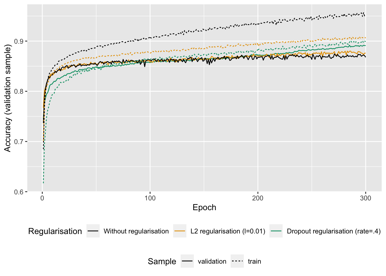
Figure 6.15: Accuracy with or without regularisation (L2 or dropout)
We note that using regularisation techniques, the model is less prone to overfitting.
6.2 Recurrent Neural Networks
This section presents models that can be used to predict sequence data. The focus will be made on time series here.
Densely connected networks as those presented earlier have no memory. In contrast, recurrent neural networks will process each training example as a sequence, it will loop over the elements of the sequence before turning to another training example. During the loop, the network will iterate over the elements of the training example (for time series, these elements will be the lagged values).
The input given the the network is a 2D tensor. The first dimension of the tensor is the time step, while the second is made of the predictors. The network loops over the time steps. At each time step \(\ell\), it considers the input values at \(\ell\) as well as some state values at time \(\ell\). The state values correspond to what the network has seen over the previous iterations of the current sequence (which is initialised to 0 for the first time step).
Each observation/example can be represented as a sequence of \(L\) points in time, so \(X_t=\{L^LX_t, \ldots, L^2X_t, LX_t\}\), where \(L\) is the lag operator such that \(LX_t=X_{t-1}\), \(L^2X_t = X_{t-2}\), and so on. The output \(Y\) is the point value to be predicted.
Figure 6.16 illustrates how a recurrent neural network operates, considering a time series with 3 lags accounted for (i.e., a sequence of length 3), where \(\color{IBMMagenta}{\mathbf{X}}\color{black} = \color{IBMMagenta}{\{L^3\mathbf{X}_t}\color{black}, \color{IBMMagenta}{L^2\mathbf{X}_t}\color{black}, \color{IBMMagenta}{L\mathbf{X}_t}\}\), an output \(Y\) to predict, and a hidden-layer sequence \(\color{IBMPurple}{\{As\}_{1}^{S}}\color{black} = \{\color{IBMPurple}{A_1}\color{black}, \color{IBMPurple}{A_2}\color{black}, \ldots, \color{IBMPurple}{A_S}\}\). Each \(\color{IBMMagenta}{\mathbf{X}_\ell}\) is a vector \([\color{IBMMagenta}{\mathbf{X}_{\ell,1}}\color{black}, \color{IBMMagenta}{\mathbf{X}_{\ell,2}}\color{black}, \ldots, \color{IBMMagenta}{\mathbf{X}_{\ell,p}}\color{black}]\).
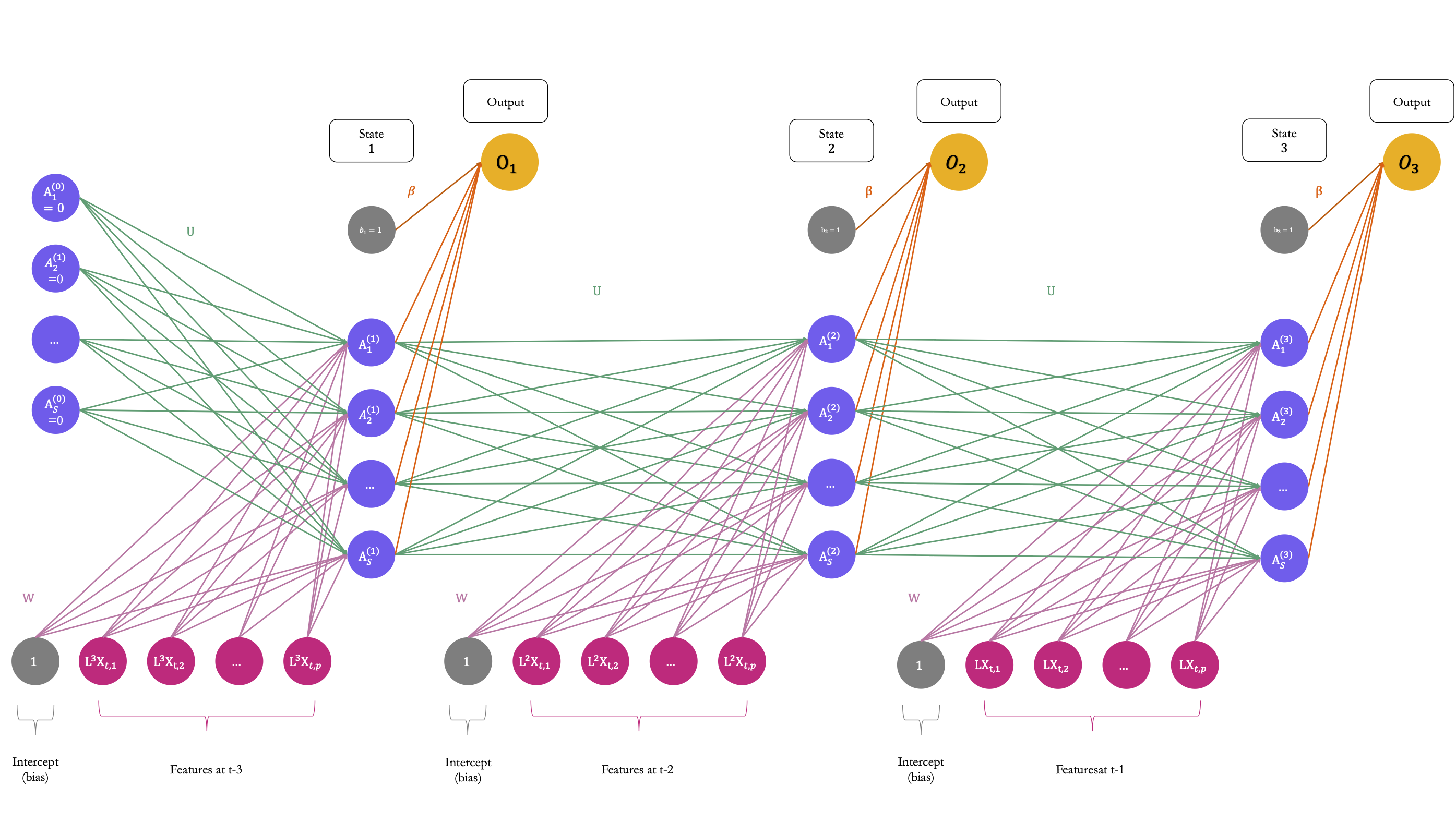
Figure 6.16: A simple recurrent neural network which processes sequences of length 3.
At each time step \(\ell\), the activations \(\color{IBMPurple}{A_1^{(\ell)}}\color{black}, \color{IBMPurple}{A_2^{(\ell)}}\color{black}, \ldots, \color{IBMPurple}{A_S^{(\ell)}}\) are updated using:
- a linear combination of the previous activations \(\color{IBMPurple}{A_1^{(\ell-1)}}\color{black}, \color{IBMPurple}{A_2^{(\ell-1)}}\color{black}, \ldots, \color{IBMPurple}{A_S^{(\ell-1)}}\) weighted by a matrix of weights \(\color{wongGreen}{\mathbf{U}}\)
- a linear combination of the inputs \(\color{IBMMagenta}{\mathbf{X}_\ell}\) weighted by a matrix of weights \(\color{wongPurple}{\mathbf{W}}\)
- and a bias (intercept) \(\color{gris}{w_{s_0}}\).
The \(s\)-th activation in time step \(\ell\), with \(k=1,\ldots, S\) writes: \[\begin{align} \color{IBMPurple}{A_{s}^{(\ell)}}\color{black} = \color{IBMPurple}{g}\color{black}\left(\color{gris}{w_{s_0}}\color{black} + \sum_{j=1}^{\color{Magenta}{p}\color{black}} \color{wongPurple}{w_{kj}} \color{IBMMagenta}{\mathbf{X}_{\ell,j}}\color{black} + \sum_{s=1}^{\color{IBMMagenta}{S}\color{black}} \color{wongGreen}{u_{ks}} \color{IBMPurple}{A_{s}^{(\ell-1)}}\color{black}\right), \end{align}\]
where \(\color{IBMPurple}A_{s}^{(0)}=0\) for all \(s=1, \ldots, S\).
Then, each activations at time step \(\ell\) is fed to the output layer:
\[\color{IBMYellow}{O_{\ell}}\color{black} = f\left(\color{gris}{\beta_0}\color{black} + \sum_{s=1}^{\color{IBMPurple}{S}} \color{wongOrange}{\beta_s}\color{IBMPurple}{A_{s}^{(\ell)}}\color{black}\right),\]
where \(\color{IBMYellow}{f}\color{black}(\cdot)\) is an activation function (the identity function for a quantitative response).
Figure 6.17 shows a more compact schematic of the same architecture as that shown in Figure 6.16.
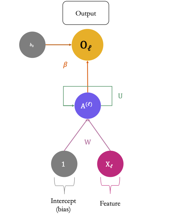
Figure 6.17: The more compact schematic of the simple recurrent neural network which processes sequences of length 3.
For a regression problem, the loss function to be optimised is the residual sum of squares: \[\sum_{i=1}^{n} \left(y_i - o_{i}^{(L)}\right)^2,\] for \(i=1,\ldots, n\), where \(o_{i}^{(L)}\) is the output for the \(i\)-th observation (the prediction).
Observe that only the last output \(O^{L}\) is used in the minimisation problem.
6.2.1 Practice with Keras
Let us return to the Seoul bike dataset. Up until now, we have ignored the fact that these data can be processed as time series. Let us follow the example on weather data provided in the 6th chapter of Chollet and Allaire (2018) and adapt it to the Seoul bike data.
First, as noticed by one of the participants during the second hands-on session, the hour variable could be considered in a more intelligent way than was done with the trees. Let us create two variables from it:
- one indicating whether is evening (from 7pm to 9pm), night (from 10pm to 6am), day (7am to 6pm)
- another one indicating whether each observation is recorded at 8 am (morning peek), 6pm (afternoon peak), or outside peak periods.
Other feature engineering could be considered, of course.
bike <-
  bike %>%
  mutate(day_moment = case_when(
    hour > 18 & hour <= 22 ~ "evening",
    hour > 22 | hour <= 6 ~ "night",
    hour > 6 & hour <= 18 ~ "day",
    TRUE ~ "problem"
  )) %>%
  mutate(day_peak = case_when(
    hour == 18 ~ "evening",
    hour == 8 ~ "morning",
    TRUE ~ "none"
  ))
Let us have a look at the distribution of those new variables:
prop.table(table(bike$day_moment))##
## day evening night
## 0.5004135 0.1668045 0.3327820prop.table(table(bike$day_peak))##
## evening morning none
## 0.04170112 0.04170112 0.91659776The data spans from 2017-12-01 to 2018-11-30:
range(bike$date)## [1] "2017-12-01" "2018-11-30"As the training, validation and test samples will be constituted while keeping the notion of temporality, it is not possible to use the variable indicating the months as a qualitative variable. There are not enough observations to include this variable in the model. The hour variable will also be discarded from the features, as two other variables were just created to avoid using the former as a numerical variable. (It could have been possible to just create dummy 11 variables from the hour variable instead.)
Let us remove the unnecessary variables from the sample, and in the mean time, let us create dummy variables for all qualitative variables.
data_bikes <-
  bike %>%
  select(-date, -y_binary, -month, -seasons, -hour) %>%
  dummy_cols(
    remove_first_dummy = TRUE,
    remove_selected_columns = TRUE)
6.2.1.1 Preparing Training, Validation and Test Datasets
The whole dataset can be split into three parts:
- the train set: from the first observation to the five-thousandth (
1:5000) - the validation set: from the five-and-a-half thousandth to the six-thousand-and-five-hundredth (
5001:6500) - the test set: the remainder
ind_train <- 1:5000
ind_valid <- 5001:6500
Let us store in an object the index of the column of the target variable in the dataset:
ind_target <- which(colnames(data_bikes) == "rented_bike_count")
ind_target
## [1] 1The observations need to be scaled, as in the previous examples, to make the optimisation problem look for solutions in a less complex dimension.
train_data <- data_bikes[ind_train, -ind_target]In order to get a better idea of the model’s capabilities when exposed to unseen data, the mean and standard deviation for scaling each explanatory variable should be calculated on the training data.
(mean <- apply(train_data, 2, mean))## temperature humidity wind_speed
## 7.659700 55.265200 1.864140
## visibility dew_point_temperature solar_radiation
## 1334.842400 -1.634220 0.537718
## rainfall snowfall year
## 0.126340 0.106920 2017.851200
## holiday_No Holiday week_day_Tue week_day_Wed
## 0.942400 0.144000 0.139200
## week_day_Thu week_day_Fri week_day_Sat
## 0.139200 0.145600 0.144000
## week_day_Sun day_moment_evening day_moment_night
## 0.144000 0.166400 0.334200
## day_peak_morning day_peak_none
## 0.041600 0.916800(std <- apply(train_data, 2, sd))## temperature humidity wind_speed
## 11.1084170 21.2841883 1.0904797
## visibility dew_point_temperature solar_radiation
## 639.5248880 12.2944269 0.8582797
## rainfall snowfall year
## 1.0224565 0.4750508 0.3559268
## holiday_No Holiday week_day_Tue week_day_Wed
## 0.2330088 0.3511248 0.3461897
## week_day_Thu week_day_Fri week_day_Sat
## 0.3461897 0.3527400 0.3511248
## week_day_Sun day_moment_evening day_moment_night
## 0.3511248 0.3724766 0.4717572
## day_peak_morning day_peak_none
## 0.1996933 0.2762119It is important to check that no standard deviation is exactly equal to 0, which could be the case if a dummy variable takes a single value in the training set and another one in the validation or the test sets. Any variable for which the standard deviation computed on the training set should therefore be removed from the features.
The data can then be scaled:
data_bikes_x <- data_bikes[, -ind_target]
data_bikes_x <- scale(data_bikes_x, center = mean, scale = std)
Let us scale the target variable a bit differently, as it is count data:
max_target <- max(data_bikes[[ind_target]])
target_bikes <- data_bikes[[ind_target]]/max_target
Let us add the target variable:
data_bikes <- cbind(target_bikes, data_bikes_x)
ind_target <- 1
To update the parameters of the model, we will rely on batches of training data. The samples will be generated on the fly. To do so, the approach provided in the 6th chapter of Chollet and Allaire (2018) will be used. Such an approach is particularly useful when the data at hand is huge and cannot be stored in memory: instead of loading all the training examples, they are loaded only when sampled to be included in a batch.
As previously stated, we will feed to model with 2D tensors. The first dimension will be the time step \(\ell\) while the second dimension will be the matrix of predictors at the corresponding time step \(\ell\).
Let us say that we want to:
- make predictions 24 hours ahead: we will set a parameter named
delayto24, as the unit of time in the bike dataset is the hour - rely on the previous 3-days data: we will set a parameter named
lookbackto3*24 - sample the observations every
steps=1time steps.
We will use a batch size of 32.
lookback <- 3*24
step <- 1
delay <- 24
batch_size <- 32
The function that generates samples expects some indices to specify where in the whole dataset to sample from. This allows us to generate batches of observations for the training sample, for the validation sample, and for the test sample. Note, however, that we will also define another function to generate all the examples from the test sample with another function, to look at the predicted values.
#' WARNING: as variable `i_gen` is updated in the
#' global environment you should make sure that no variable
#' with the same name is used in your code.
#' Otherwise, some conflicts may appear.
#' Function from Chollet & Allaire (2018)
#' @param data Data frame with all the observations in rows
#' @param lookback Number of lags
#' @param delay Horizon for the prediction
#' @param min_index,max_index Index of the first and last
#'                  examples in `data` in which sampling
#'                   is to take place
#' @param shuffle Should the rows of the dataset from which
#'                samples are drawn be randomly swapped before
#'                sampling?
#' @param batch_size Number of samples per batch
#' @param step Period, in time steps, at which samples are drawn
#'             for daily data, if `step=3`, samples are drawn
#'             every 3 days
#' @param ind_target col index of the target variable in `data`
generator <-
  function(data, lookback, delay, min_index, max_index,
           shuffle = FALSE, batch_size = 128, step = 6,
           ind_target) {
    if (is.null(max_index))
      max_index <- nrow(data) - delay - 1

    i_gen <- min_index + lookback
    function() {
      if (shuffle) {
        rows <- sample(c((min_index+lookback):max_index),
                       size = batch_size)
      } else {
        if (i_gen + batch_size >= max_index)
          i_gen <<- min_index + lookback
        rows <- c(i_gen:min(i_gen+batch_size, max_index))
        i_gen <<- i_gen + length(rows)
      }
      samples <- array(0, dim = c(length(rows),
                                  lookback / step,
                                  dim(data)[[-1]]))
      targets <- array(0, dim = c(length(rows)))
      # targets_j <- array(0, dim = c(length(rows)))
      for (j in 1:length(rows)) {
        indices <- seq(rows[[j]] - lookback, rows[[j]],
                       length.out = dim(samples)[[2]])
        samples[j,,] <- data[indices,]
        targets[[j]] <- data[rows[[j]] + delay, ind_target]
        # targets_j[[j]] <- rows[[j]] + delay
      }
      list(samples, targets)
    }
}
The generator() function returns a list with two elements:
samples: the observations sampled, stored in an array of dimensions [batch_size,lookback,number_of_predictors], wherenumber_of_predictorsis, as you surely already guessed, the number of predictorstargets: the vector of the corresponding targets for thebatch_sizeexamples drawn.
Let us define an object that will draw observations from the training set when it will be called during the training of the network:
train_gen <- generator(
  data = data_bikes,
  lookback = lookback,
  delay = delay,
  min_index = 1,
  max_index = max(ind_train),
  shuffle = TRUE,
  step = step,
  batch_size = batch_size,
  ind_target = ind_target
)
The same can be done for the objects that will draw observations from the validation set, and for the test set:
val_gen <- generator(
  data = data_bikes,
  lookback = lookback,
  delay = delay,
  min_index = min(ind_valid),
  max_index = max(ind_valid),
  shuffle = FALSE,
  step = step,
  batch_size = batch_size,
  ind_target = ind_target
)

test_gen <- generator(
  data = data_bikes,
  lookback = lookback,
  delay = delay,
  min_index = max(ind_valid)+1,
  max_index = NULL,
  shuffle = FALSE,
  step = step,
  batch_size = batch_size,
  ind_target = ind_target
)
You may have noticed that for val_gen() and test_gen(), the argument shuffle was set to FALSE. We can thus have an idea of how many steps are needed to draw from these functions in order to see the entire validation and entire set, respectively.
val_steps <-
  (max(ind_valid)-min(ind_valid)-lookback)/batch_size
val_steps
## [1] 44.59375test_steps <-
(nrow(data_bikes)-(max(ind_valid)+1)-lookback)/batch_size
test_steps## [1] 59.125As mentioned earlier, we can also create a function to create the complete set of tensors from the training sample:
generate_data_full <-
  function(data, lookback, delay, min_index, max_index,
           step = 1, ind_target) {

    rows_min <- max(min_index, lookback)
    rows_max <- max_index-delay
    rows <- rows_min:rows_max
    function(){
      samples <-
        array(0, dim = c(length(rows),
                         lookback / step,
                         dim(data)[[-1]]))
      targets <- array(0, dim = c(length(rows)))
      for (j in 1:length(rows)) {
        indices <-
          seq(rows[[j]] - (lookback-1), rows[[j]],
              length.out = dim(samples)[[2]])
        samples[j,,] <- data[indices,]
        targets[[j]] <- data[rows[[j]]+delay, ind_target]
      }
      list(samples, targets)
    }
  }
This generate_data_full() works in the same spirit as the previous generation function, except that it does not perform sampling.
The positions of the values in the training sample can be stored:
ind_test <- (last(ind_valid)+1):nrow(data_bikes)Let us also create an object that will contain the generate_data_full() function and will return a list with two elements:
samples: the test examples, stored in an array of dimensions [n_test,lookback,number_of_predictors], wheren_testcorresponds to the number of observations in the test sample minusdelay.targets: the corresponding values of the target variable.
data_test <-
  generate_data_full(
    data = data_bikes,
    lookback = lookback,
    delay = delay,
    min_index = ind_test[1],
    max_index = last(ind_test),
    step = 1,
    ind_target = ind_target
  )
Let us create the tensors containing the all the observations from the test sample:
c(x_data_test, y_data_test) %<-% data_test()There are 1941 observations and 21 predictors, for which the past 72 values are stored (from earliest to latest date).
dim(x_data_test)## [1] 1941 72 21There are 1941 corresponding target values:
dim(y_data_test)## [1] 19416.2.1.2 Naive Benchmark
Assume that the number of bikes rented per hour is a continuous variable (which is debatable, since it is actually count data). Further assume that the number of bikes rented is periodical with a daily period. Then you can assume that the number of bikes rented at the same time the next day will be identical to the number of bikes rented now. Under these asumption, what would the mean absolute error be?
#' Computes the average of MAE obtained on batches drawn
#' from the validation sample.
#' The number of batches drawn is `val_steps`
#' Function from Chollet & Allaire (2018)
evaluate_naive_method <- function() {
  batch_maes <- rep(NA, val_steps)
  for (step in 1:val_steps) {
    # Gen. batches of data from the validation sample
    c(samples, targets) %<-% val_gen()
    # Take the last observed values for each example
    # in the batch, i.e., target_{t-1}
    preds <- samples[, dim(samples)[[2]], ind_target]
    # CMAE using target_{t-1} as the predicted value
    mae <- mean(abs(preds - targets))
    batch_maes[step] <- mae
  }
  # Avg of MAE obtained over the different batches
  mean(batch_maes)
}
batch_mae <- evaluate_naive_method()
batch_mae
## [1] 0.0748107The average absolute error, under these hypotheses would therefore be equal to 266.03:
batch_mae*max_target## [1] 266.0269Can a recurrent neural network beat this? Easier said than done.
6.2.1.3 A Densely Connected Model
In a first step, let us try to predict the number of rented bikes with a simple densely connected model. A recurrent neural network will be trained after and the predictive capacities on the validation sets can be compared.
Let us use a single hidden layer with 16 units. The data will be flatten using the layer_flatten() function. Hence, the lagged values will be used as predictors, but the model will not consider that the data are sequential. As the target variable is numerical with values in \(\mathbb{R}^{+}\), let us use a ReLU activation in the output layer.
model_benchmark <-
  keras_model_sequential() %>%
  layer_flatten(
    input_shape = c(lookback / step, dim(data_bikes)[-1])) %>%
  layer_dense(units = 16, activation = "relu") %>%
  layer_dense(units = 1, activation = "relu")
The loss function that will be used is the MAE.
model_benchmark %>% compile(
  optimizer = "rmsprop",
  loss = "mae"
)
The model can be trained over 50 epochs. At each epoch, 60 batches of data will be drawn from the generator. The MAE will also be computed on val_steps.{R}=44.59375 validation samples drawn from the generator.
history_benchmark <-
  model_benchmark %>%
  fit(
    train_gen,
    steps_per_epoch = 60,
    epochs = 50,
    validation_data = val_gen,
    validation_steps = val_steps
  )
The results can be saved:
model_benchmark %>%
  save_model_hdf5(
    "deep_learning_models/bikes_model_benchmark.h5")
save(history_benchmark,
     file =
       "deep_learning_models/history_benchmark.rda")
Let us have a look at the MAE computed both on the training and the validation sets during the training.
plot(history_benchmark)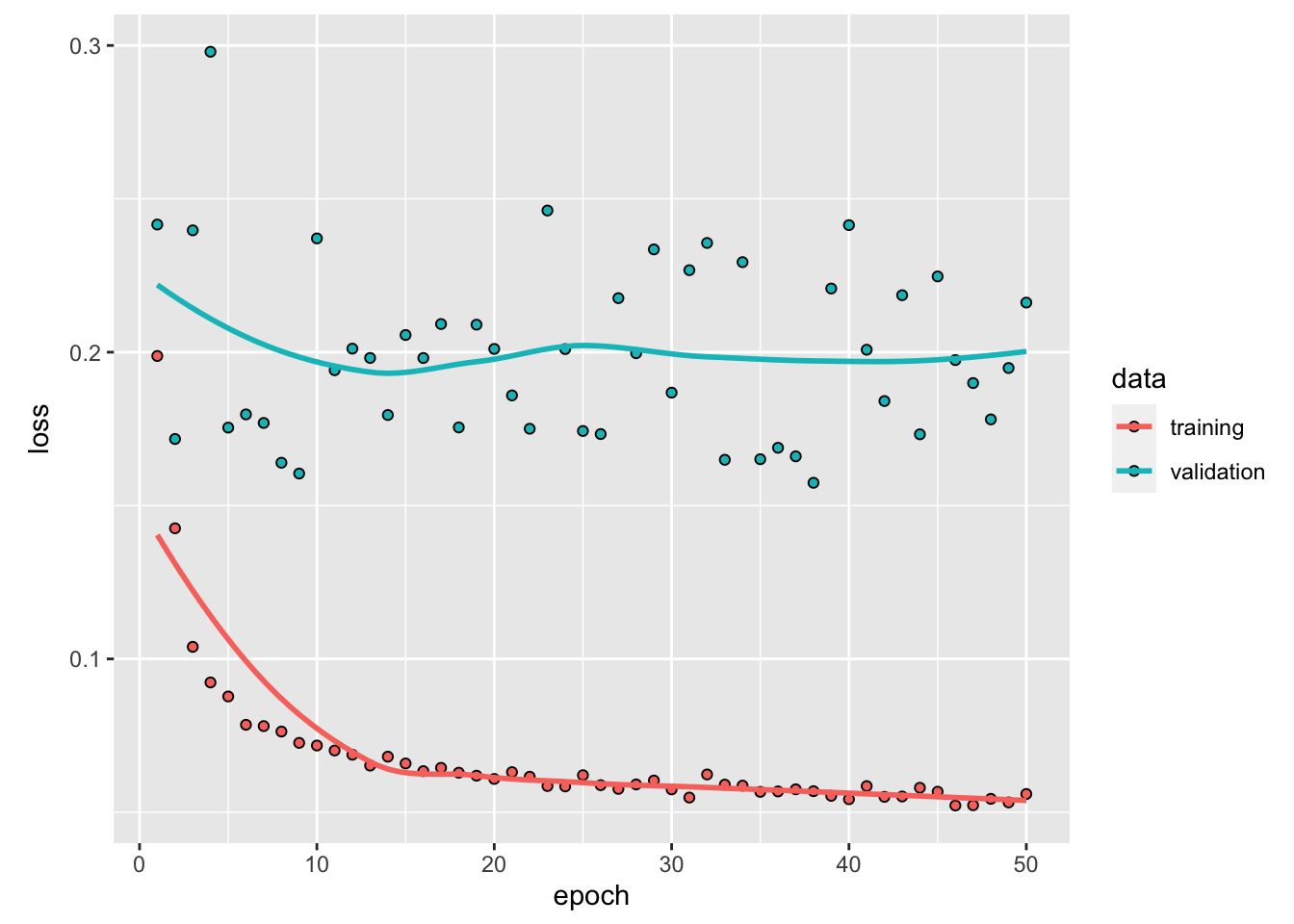
Figure 6.18: Training and validation MAE on bike data, with the densely connected network.
The results obtained with both the training and validation samples are quite poor. In addition, the model overfits.
The MAE on the test set:
mae_nn <-
  evaluate(model_benchmark, x=x_data_test, y=y_data_test)
mae_nn*max_target
## loss
## 506.5381We have poor performances on the test set here.
The predictions on the test set can be obtained as follows (recall the x_data_test was created earlier):
preds_nn <- predict(model_benchmark, x = x_data_test)Let us have a look at the predicted values hour by hour over the test sample.
ind_in_data <- ind_test[(delay+1):length(ind_test)]
df_test_pred_nn <-
  tibble(obs = bike$rented_bike_count[ind_in_data],
         pred = preds_nn[,1]*max_target) %>%
  mutate(date = bike$date[ind_in_data],
         hour = bike$hour[ind_in_data],
         hm = lubridate::ymd_h(str_c(date, " ", hour))
         ) %>%
  mutate(month = lubridate::month(date))
Let us plot the results:
df_test_pred_nn %>%
  pivot_longer(cols = c(obs, pred),
               names_to = "type", values_to = "bike") %>%
  ggplot(data = .,
         mapping = aes(x = hm, y = bike,
                       colour = type, linetype = type)) +
  geom_line() +
  facet_wrap(~month, scale = "free", ncol=1) +
  labs(x = "Date", y = "Number of rented bikes") +
  scale_colour_manual(
    NULL,
    values = c("obs" = "#648FFF", "pred" = "#DC267F")) +
  scale_linetype_discrete(NULL)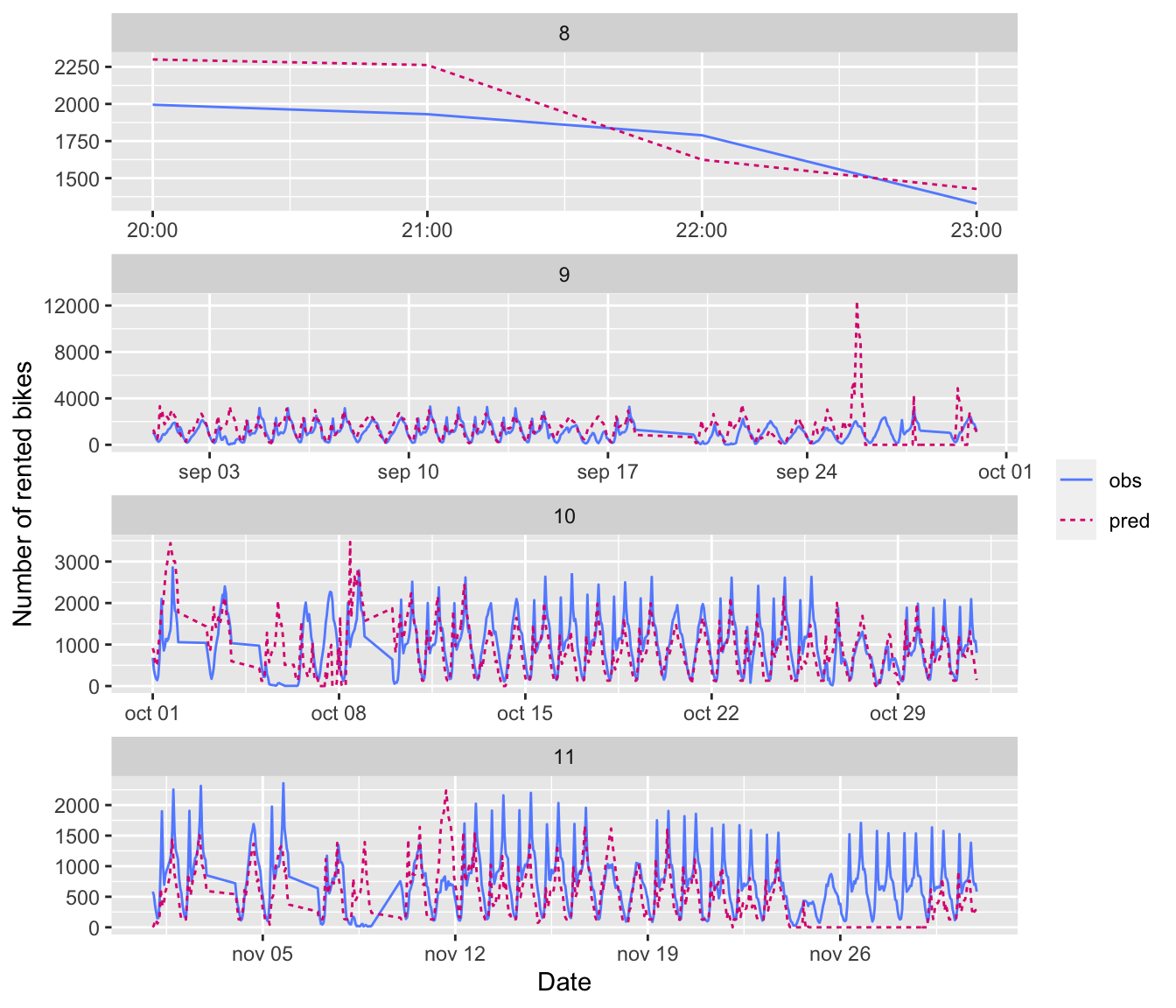
Figure 6.19: Predictions for the densely connected network, by month.
We can also look at the residuals:
df_test_pred_nn %>%
  mutate(residuals = obs-pred) %>%
  ggplot(data = ., mapping = aes(x=hm, y = residuals)) +
  geom_line() +
  geom_hline(yintercept = 0, colour = "#648FFF",
             linetype = "dashed") +
  labs(x = "Date", y = "Residuals")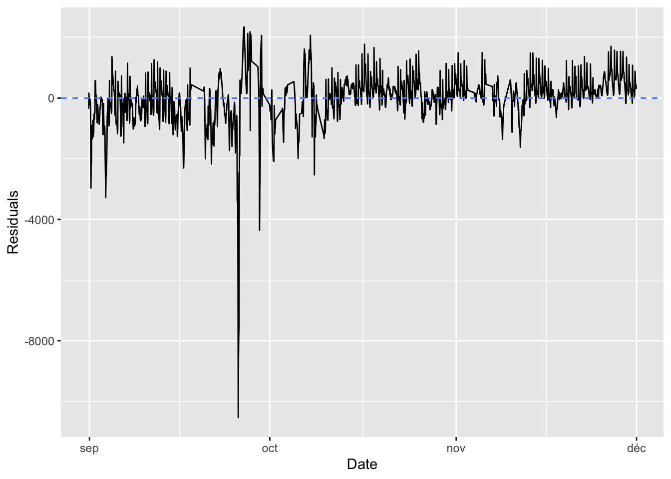
Figure 6.20: Residuals for the densely connected network, estimations made on the test sample.
6.2.1.4 Recurrent Network without Dropout
Now, let us consider the data as sequential and build our first recurrent network. We will use the GRU layer (Gated recurrent unit), as in the example from Chollet and Allaire (2018), and as in Emanuelle Flachaire’s course.
model_rnn <-
  keras_model_sequential() %>%
  layer_gru(
    units = 16,
    input_shape = list(NULL, dim(data_bikes)[[-1]])) %>%
  layer_dense(units = 1, activation = "relu")
The MAE will once again be the loss function being optimised:
model_rnn %>%
  compile(
    optimizer = "rmsprop",
    loss = "mae"
  )
The model can be trained over 50 epochs, drawing 60 batches per epoch. At each epoch, 44.59375 batch samples will be drawn from the validation set, and the MAE will be computed on those samples.
history_rnn <-
  model_rnn %>%
  fit(
    train_gen,
    steps_per_epoch = 60,
    epochs = 50,
    validation_data = val_gen,
    validation_steps = val_steps
  )
Once the model is estimated, it can be saved.
model_rnn %>% save_model_hdf5("deep_learning_models/model_rnn.h5")
save(history_rnn, file = "deep_learning_models/history_rnn.rda")
Let us have a look at the MAE over the epochs.
plot(history_rnn)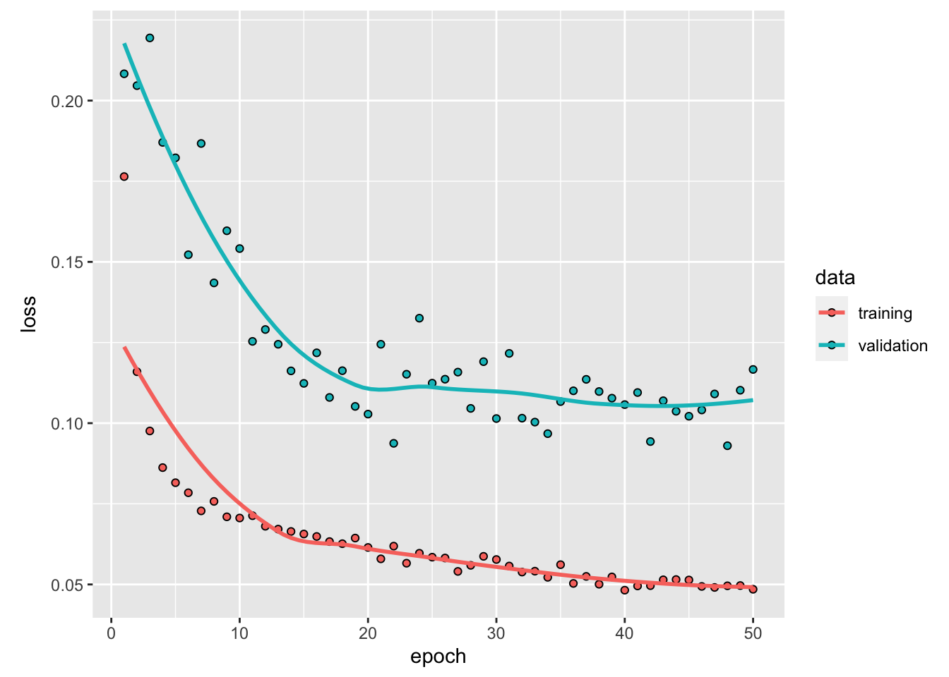
Figure 6.21: Training and validation MAE on bike data, with the first recurrent network.
The performances seem almost correct here (maybe a bit more epochs could lead to lower MAE on the validation set: the algorithm does not seem to have converged yet). We note that the model overfits.
The performances of the model on the test data can be assessed as well:
mae_rnn <- evaluate(model_rnn, x=x_data_test, y=y_data_test)
mae_rnn*max_target
## loss
## 280.2893Not so bad.
The predictions using that model can be obtained as follows:
preds_rnn <- predict(model_rnn, x=x_data_test)Let us put those predicted values in a tibble:
ind_in_data <- ind_test[(delay+1):length(ind_test)]
df_test_pred_rnn <-
  tibble(obs = bike$rented_bike_count[ind_in_data],
         pred = preds_rnn[,1]*max_target) %>%
  mutate(date = bike$date[ind_in_data],
         hour = bike$hour[ind_in_data],
         hm = lubridate::ymd_h(str_c(date, " ", hour))
         ) %>%
  mutate(month = lubridate::month(date))
The predicted values and the observed values on the test sample can be plotted:
df_test_pred_rnn %>%
  pivot_longer(cols = c(obs, pred),
               names_to = "type", values_to = "bike") %>%
  ggplot(data = .,
         mapping = aes(x = hm, y = bike,
                       colour = type, linetype = type)) +
  geom_line() +
  facet_wrap(~month, scale = "free", ncol=1) +
  labs(x = "Date", y = "Number of rented bikes") +
  scale_colour_manual(
    NULL,
    values = c("obs" = "#648FFF", "pred" = "#DC267F")) +
  scale_linetype_discrete(NULL)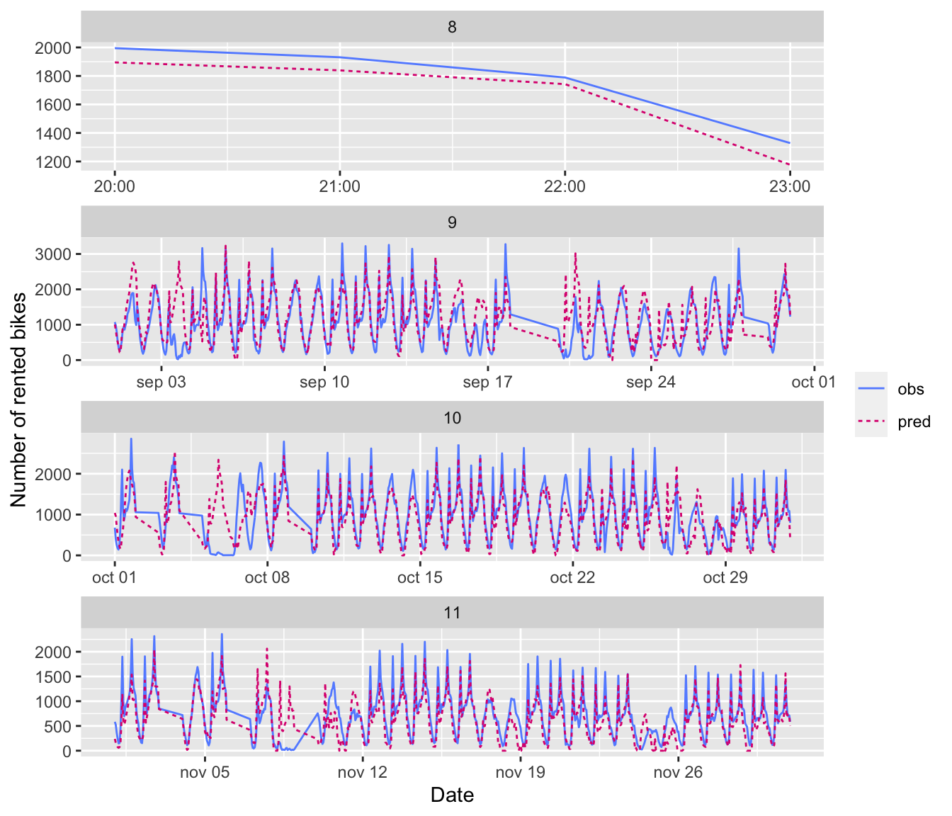
Figure 6.22: Predictions for the first recurrent network, by month.
Let us look at the residuals:
df_test_pred_rnn %>%
  mutate(residuals = obs-pred) %>%
  ggplot(data = ., mapping = aes(x=hm, y = residuals)) +
  geom_line() +
  geom_hline(yintercept = 0, colour = "#648FFF",
             linetype = "dashed") +
  labs(x = "Date", y = "Residuals")
Figure 6.23: Residuals with the first recurrent network.
The model tends to underestimate the number of rented bikes at the end og the period. Having more data to capture seasonnal patterns over the year may help.
6.2.1.5 Recurrent Network with Dropout
We observe some overfitting with the previous recurrent network. Let us try to fight it using dropout. As explained in Chollet and Allaire (2018), with recurrent neural networks, the activations that are temporarily set to 0 should be the same for every time step (to propagate the learning error through time). Such a mechanisme is already in use in Keras. The argument dropout of a layer controls the dropout rate applied to this layer. In addition, a dropout rate can be applied to the recurrent activations of a layer (the \(A_s^{(\ell-1)}\)): a temporally constant mask should be used. The dropout rate of the recurrent activations is controlled by the argument recurrent_dropout of the layer.
model_rnn_drop <-
  keras_model_sequential() %>%
  layer_lstm(
    units = 16,
    dropout = 0.3,
    recurrent_dropout = 0.4,
    input_shape = list(NULL, dim(data_bikes)[[-1]])) %>%
  layer_dense(units = 1, activation = "relu")
Once again, the loss function is the MAE:
model_rnn_drop %>% compile(
  optimizer = "rmsprop",
  loss = "mae"
)
Networks for which regularisation methods are applied usually need mode epochs to converge. A rule of thumb is to aim about twice the number of epochs.
history_rnn_drop <-
  model_rnn_drop %>%
  fit(
    train_gen,
    steps_per_epoch = 60,
    epochs = 100,
    validation_data = val_gen,
    validation_steps = val_steps
  )
The trained model can be saved:
model_rnn_drop %>%
  save_model_hdf5("deep_learning_models/model_rnn_drop.h5")
save(history_rnn_drop,
     file = "deep_learning_models/history_rnn_drop.rda")
Let us have a look at the evolution of the MAE over the training process:
plot(history_rnn_drop)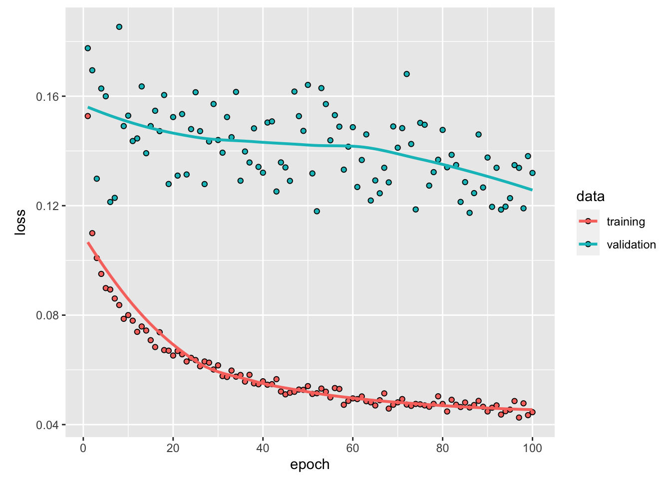
Figure 6.24: Training and validation MAE on bike data, with the regularised recurrent network.
The model still overfits and the predictions are not very good.
The MAE on the test set:
mae_rnn_drop <-
  evaluate(model_rnn_drop,
           x=x_data_test, y=y_data_test)
mae_rnn_drop*max_target
## loss
## 314.8936Let us make some prediction using the model:
preds_rnn_drop <-
  predict(model_rnn_drop, x = x_data_test)
Let us put those predicted values in a tibble:
ind_in_data <- ind_test[(delay+1):length(ind_test)]
df_test_pred_rnn_drop <-
  tibble(obs = bike$rented_bike_count[ind_in_data],
         pred = preds_rnn_drop[,1]*max_target) %>%
  mutate(date = bike$date[ind_in_data],
         hour = bike$hour[ind_in_data],
         hm = lubridate::ymd_h(str_c(date, " ", hour))
         ) %>%
  mutate(month = lubridate::month(date))
The predicted values and the observed values on the test sample can be plotted:
df_test_pred_rnn_drop %>%
  pivot_longer(cols = c(obs, pred),
               names_to = "type", values_to = "bike") %>%
  ggplot(data = .,
         mapping = aes(x = hm, y = bike,
                       colour = type, linetype = type)) +
  geom_line() +
  facet_wrap(~month, scale = "free", ncol=1) +
  labs(x = "Date", y = "Number of rented bikes") +
  scale_colour_manual(
    NULL,
    values = c("obs" = "#648FFF", "pred" = "#DC267F")) +
  scale_linetype_discrete(NULL)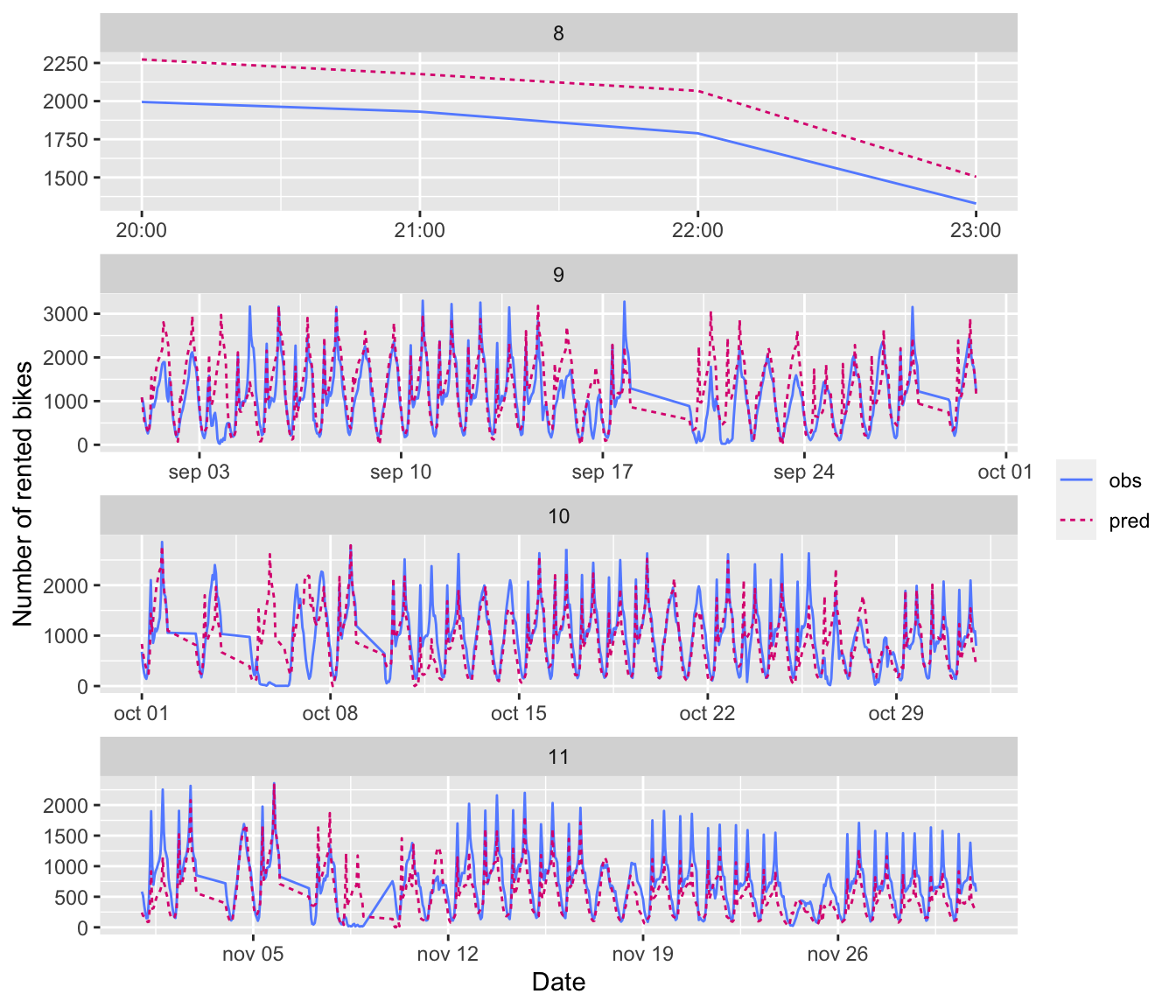
Figure 6.25: Predictions for the regularised recurrent network, by month.
The model still underestimate the needs at the end of the period.
df_test_pred_rnn_drop %>%
  mutate(residuals = obs-pred) %>%
  ggplot(data = ., mapping = aes(x=hm, y = residuals)) +
  geom_line() +
  geom_hline(yintercept = 0, colour = "#648FFF",
             linetype = "dashed") +
  labs(x = "Date", y = "Residuals")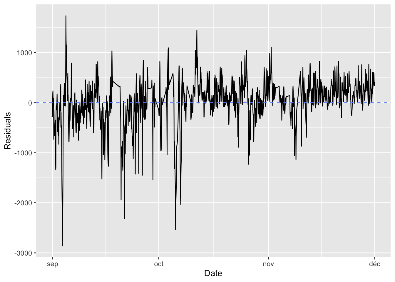
Figure 6.26: Residuals with the regularised recurrent network.
The models that were trained need to be fine tuned to get better results. But to better account for the cyclical components of the data over the year, multiple years are needed.
Now it is your turn: compare the performances obtained with a neural network and those obtained with an ARIMA model.