2 Gradient Descent

This chapter presents the gradient descent algorithm used to optimise functions. It begins with the vanilla version of the gradient descent algorithm, then moves to variants (stochastic gradient descent, batch gradient descent, mini-batch gradient descents). It end with two other techniques: Newton’s method and coordinate descent algorithm.

2.1 Vanilla Gradient Descent

2.1.1 Concept

Let us consider a very general model:

\[y = m(\boldsymbol{X}) + \varepsilon,\] where $y$ is a variable to predict (or target variable, or response variable), $m(\cdot)$ is an unknown model, $\boldsymbol{X}$ is a set of $p$ predictors (or features, or inputs, or explanatory variables) and $\varepsilon$ is an error term.

Let us assume that the response variable is linearly dependent on the set of explanatory variables: \[y = \boldsymbol{X}\beta + \varepsilon,\]

We do not know the true generating data process and only observe some realizations of $y$ and $\boldsymbol{X}$ for $n$ examples (or observations, or individuals). We need to make an assumption on the distribution of the error term to estimate the vector of coefficients$\beta$.

With linear least squares, we assume that the error term is normally distributed with zero mean and standard error $\sigma$. The vector of coefficients $\beta$ can be estimated with Ordinary Least Squares (OLS). The OLS estimates are such that they minimise the the sum of squared residuals, i.e., the squared difference between the observed values $y_i$ and the values predicted by the model $f(\boldsymbol{X_i})$:

\[RSS = \sum_{i=1}^{n} \left( y_i - f(\boldsymbol{X_i})\right)^2,\] where $i=1,\ldots,n$ denotes the examples (or individuals, or observations).

The problem boils down to estimating the coefficients of vector $\beta$ which minimise an objective function:

\[\text{arg}\min_\beta \sum_{i=1}^{n}\mathcal{L}\left(y_i, f(\boldsymbol{X_i})\right),\] where here: \[\mathcal{L}\left(y_i, f(\boldsymbol{X_i})\right) = \left( y_i - f(\boldsymbol{X_i})\right)^2\]

Here, with OLS, an analytical solution exists: \[\hat{\beta} = \left(\boldsymbol{X}^t\boldsymbol{X}\right)^{-1} \boldsymbol{X}^ty.\]

In a more general case, if we do not assume that the response variable is linearly dependent on the set of explanatory variables, the aim is to find the solution $\hat{m}$ to the following optimization problem: \[\text{minimise}_m \sum_{i=1}^{n} \mathcal{L}\left(y_i, m(\boldsymbol{X_i})\right).\]

The Gradient Descent algorithm is a popular technique that performs this kind of optimisation task, when the function to optimize is convex and differentiable.

2.1.2 A First Example in Dimension 1

If we know the functional form of the objective function, it is easy to find its minimum. As an illustration, consider the following function $\mathcal{L}(x) = 3x^2 - 2x + 5$.

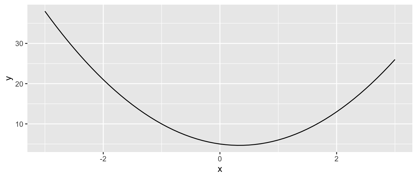
Figure 2.1: Minimising a simple loss function with a single input.

The value of $x$ that minimises this function is obtained by canceling the first derivative of $\mathcal{L}(\cdot)$ with respect to $x$, i.e.: \[\frac{\partial \mathcal{L}}{\partial x}(x) = 6x-2=0,\] which is $x=1/3$:

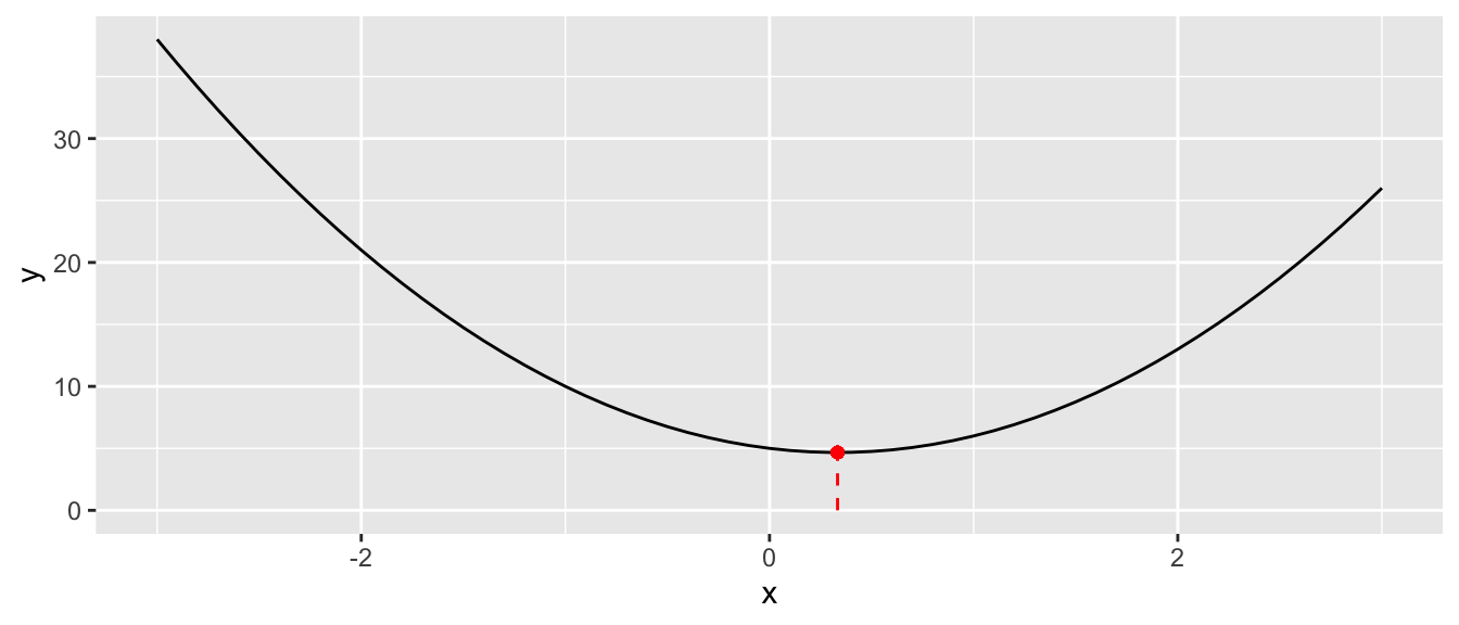
Figure 2.2: Function with a single input: minimum.

But with more complex functions, finding the minimum is not always feasible. Let us illustrate this with a simple example.

Let us consider the following function: $f(x) = (x+3) \times (x-2)^2 \times (x+1)$. The global minimum of that function is reached in $x=-1-\sqrt{\frac{3}{2}}$. Let us generate some values from this process, for $x\in [-3,3]$.

x <- seq(-3, 3, by = .1)
f <- function(x) (x+3)*(x-2)^2*(x+1)
y <- f(x)
df <- tibble(x = x, y = y)
df

## # A tibble: 61 × 2
##        x      y
##    <dbl>  <dbl>
##  1  -3     0   
##  2  -2.9  -4.56
##  3  -2.8  -8.29
##  4  -2.7 -11.3 
##  5  -2.6 -13.5 
##  6  -2.5 -15.2 
##  7  -2.4 -16.3 
##  8  -2.3 -16.8 
##  9  -2.2 -16.9 
## 10  -2.1 -16.6 
## # … with 51 more rows

Here is a graph of this function.

ggplot(data = df, aes(x=x, y=y)) +
  geom_line() +
  geom_segment(
    data = tibble(x = -1-sqrt(3/2), xend = -1-sqrt(3/2),
                  y = -Inf, yend = f(-1-sqrt(3/2))),
    mapping = aes(x = x, y=y, xend=xend, yend = yend),
    colour = "red", linetype = "dashed") +
  geom_point(x=-1-sqrt(3/2), y = f(-1-sqrt(3/2)), colour = "red")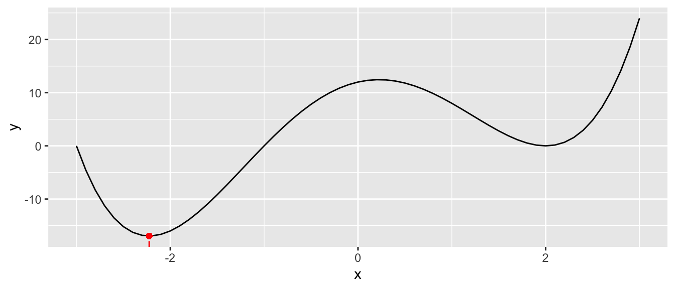

Figure 2.3: Function with a single input: a more complex function.

If we want to minimise this function using gradient descent, we can proceed as follows. In a first step, we start at a random point:

starting_value <- -.5
f(starting_value)

## [1] 7.8125

ggplot(data = df, aes(x=x, y=y)) +
  geom_line() +
  geom_point(x=starting_value, y = f(starting_value), colour = "red")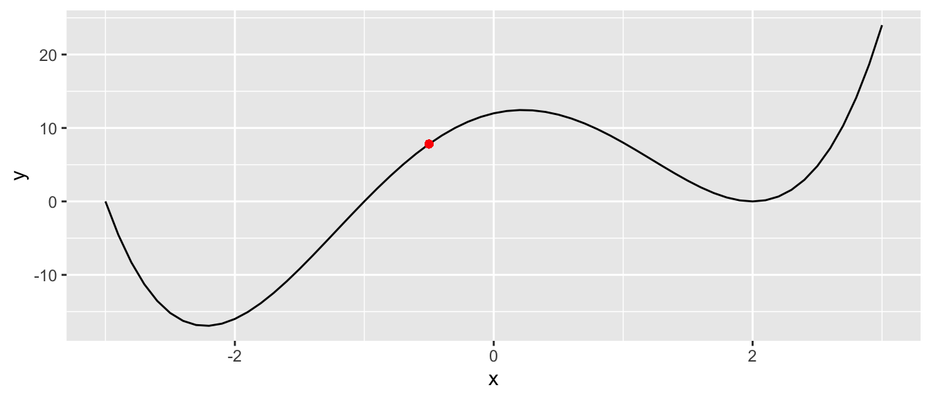

Figure 2.4: Function with a single input: start at a random point.

Then, from that point, we need to decide on two things so as to reduce the objective function:

in which direction to go next (left or right)
and how far we want to go.

To decide the direction, wan can compute the derivative of the function at this specific point of interest. The slope of the derivative will guide us:

if it is positive: we need to shift to the left
if it is negative: we need to shift to the right.

The first derivative can be obtained by numerical approximation, using the grad() function from {numDeriv}.

library(numDeriv)
grad <- grad(func = f, x = c(starting_value))
grad

## [1] 12.5

The intercept of the derivative can be computed as follows. We need it for the graph only, we could avoid computing it during the minimisation process.

(intercept <- -grad*starting_value + f(starting_value))

## [1] 14.0625

ggplot(data = df, aes(x=x, y=y)) +
  geom_line() +
  geom_point(x=starting_value, y = f(starting_value), colour = "red") +
  geom_abline(slope = grad, intercept = intercept, colour = "blue")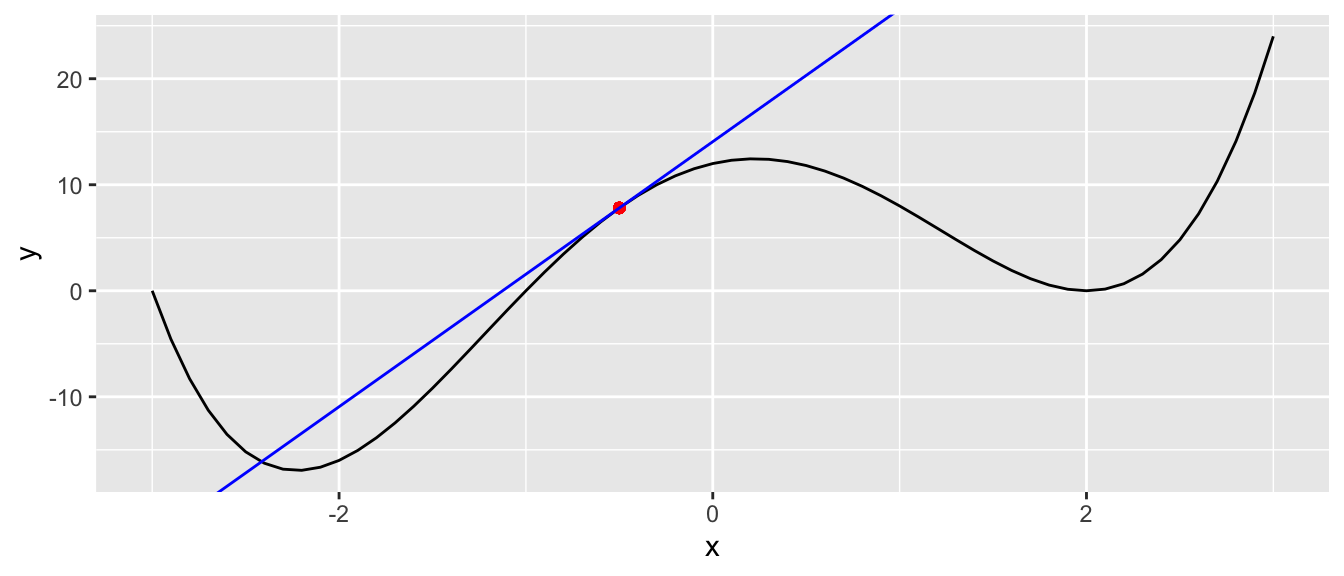

Figure 2.5: Compute the derivative of the function at that point.

Here, the slope is positive We thus need to go left We still need to decide how far we want to go, i.e., we must decide the size of the step we will take. This step is called the learning rate. On the one hand, if this learning rate is too small, we increase the risk of ending up in a local minimum; on the other hand, if we pick a too large value for the learning rate, we face a risk of overshooting the minimum and keeping bouncing around a (local) minimum forever.

Let us first pick a small value for the learning rate:

learning_rate <- 10^-2

Once we have both the direction and the magnitude of the step, we can update our parameter:

(x_1 <- starting_value - learning_rate * grad)

## [1] -0.625

ggplot(data = df, aes(x=x, y=y)) +
  geom_line() +
  geom_point(x=starting_value, y = f(starting_value), colour = "red") +
  geom_point(x=x_1, y = f(x_1), colour = "green")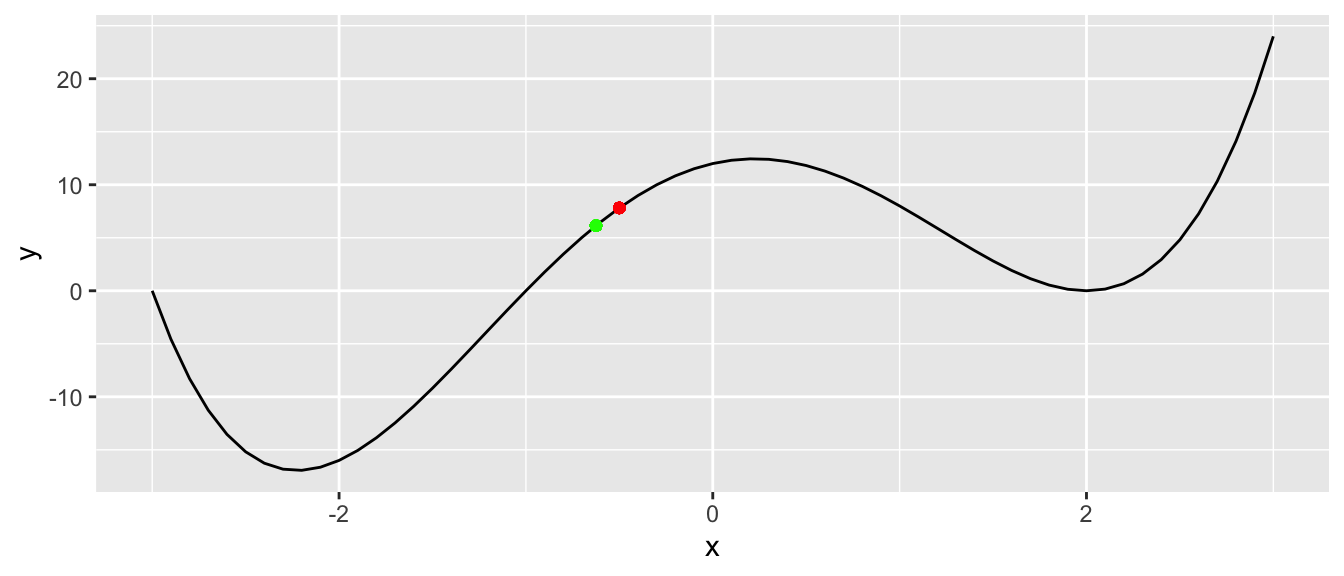

Figure 2.6: Second iteration.

Then, we can repeat the procedure mulltiple times. Let us do it through a loop. We will update our parameter from one iteration to the other and will stop either when a maximum number of iterations is reached or when the improvement (reduction in the objective function from one step to the next) is too small (below a threshold we will call tolerance).

nb_max_iter <- 100
tolerance <- 10^-5

x_1 <- -.5
# To keep track of the values through the iterations
x_1_values <- x_1
y_1_values <- f(x_1)
gradient_values <- NULL
intercept_values <- NULL

for(i in 1:nb_max_iter){
  # Steepest ascent:
  grad <- grad(func = f, x = c(x_1))
  
  intercept_value <- -grad*x_1 + f(x_1)
  # Keeping track
  gradient_values <- c(gradient_values, grad)
  intercept_values <- c(intercept_values, intercept_value)
  
  # Updating the value
  x_1 <- x_1 - learning_rate * grad
  y_1 <- f(x_1)
  
  # Keeping track
  x_1_values <- c(x_1_values, x_1)
  y_1_values <- c(y_1_values, y_1)
  
  # Stopping if no improvement (decrease of the cost function too small)
  if(abs(y_1_values[i] - y_1 < tolerance)) break
  
}

If we exit the loop before the maximum number of iterations has been reached, we can suppose we ended up in a (at least local) minimum. Otherwise, the algorithm did not converge.

## [1] 22

ifelse(i < nb_max_iter,
       "The algorithm converged.",
       "The algorithm did not converge.")

## [1] "The algorithm converged."

Let us put the computed derivative and intercept at each step in a tibble, to have a look at a graphical representation of the iterations:

df_plot <- 
  tibble(x_1 = x_1_values[-length(x_1_values)],
         y = f(x_1),
         gradient = gradient_values,
         intercept = intercept_values
  )
df_plot

## # A tibble: 22 × 4
##       x_1      y gradient intercept
##     <dbl>  <dbl>    <dbl>     <dbl>
##  1 -0.5     7.81    12.5      14.1 
##  2 -0.625   6.14    14.3      15.1 
##  3 -0.768   3.97    16.0      16.3 
##  4 -0.928   1.28    17.5      17.5 
##  5 -1.10   -1.88    18.5      18.5 
##  6 -1.29   -5.33    18.6      18.7 
##  7 -1.47   -8.73    17.7      17.4 
##  8 -1.65  -11.7     15.7      14.2 
##  9 -1.81  -14.0     12.9       9.35
## 10 -1.94  -15.4      9.79      3.52
## # … with 12 more rows

ggplot() +
  geom_line(data = df, aes(x = x, y = y)) +
  geom_point(data = df_plot, aes(x = x_1, y= f(x_1)),
             colour = "red", size = 2) +
  coord_cartesian(ylim = c(-20, 20))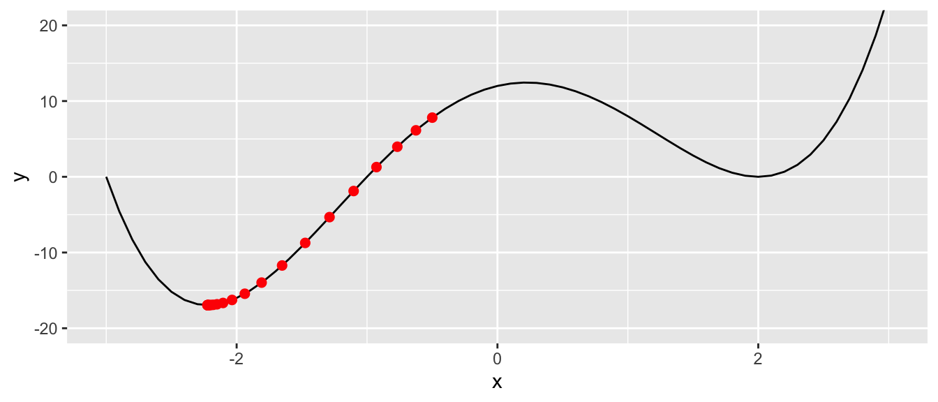

Figure 2.7: At the last step of the iteration process.

Now, let us run the same algorithm, but picking a larger value for the learning rate. Let us also increase the number of maximum iterations.

learning_rate <- 0.05
nb_max_iter <- 1000
tolerance <- 10^-5
# Starting value
x_1 <- -.5
# To keep track of the values through the iterations
x_1_values <- x_1
y_1_values <- f(x_1)
gradient_values <- NULL
intercept_values <- NULL

for(i in 1:nb_max_iter){
  # Steepest ascent:
  grad <- grad(func = f, x = c(x_1))
  
  intercept_value <- -grad*x_1 + f(x_1)
  # Keeping track
  gradient_values <- c(gradient_values, grad)
  intercept_values <- c(intercept_values, intercept_value)
  
  # Updating the value
  x_1 <- x_1 - learning_rate * grad
  y_1 <- f(x_1)
  
  # Keeping track
  x_1_values <- c(x_1_values, x_1)
  y_1_values <- c(y_1_values, y_1)
  
  # Stopping if no improvement (decrease of the cost function too small)
  if(abs(y_1_values[i] - y_1) < tolerance) break
  
}

## [1] 1000

ifelse(i < nb_max_iter,
       "The algorithm converged.",
       "The algorithm did not converge.")

## [1] "The algorithm did not converge."

df_plot <- 
  tibble(x_1 = x_1_values[-length(x_1_values)],
         y = f(x_1),
         gradient = gradient_values,
         intercept = intercept_values
  )
df_plot

## # A tibble: 1,000 × 4
##      x_1      y gradient intercept
##    <dbl>  <dbl>    <dbl>     <dbl>
##  1 -0.5    7.81    12.5      14.1 
##  2 -1.12  -2.29    18.6      18.6 
##  3 -2.05 -16.4      6.35     -3.34
##  4 -2.37 -16.5     -6.60    -32.1 
##  5 -2.04 -16.3      6.76     -2.52
##  6 -2.38 -16.4     -6.98    -33.0 
##  7 -2.03 -16.2      7.12     -1.78
##  8 -2.38 -16.4     -7.32    -33.8 
##  9 -2.02 -16.1      7.43     -1.15
## 10 -2.39 -16.3     -7.60    -34.5 
## # … with 990 more rows

ggplot() +
  geom_line(data = df, aes(x = x, y = y)) +
  geom_point(data = df_plot, aes(x = x_1, y= f(x_1)),
             colour = "red", size = .2) +
  coord_cartesian(ylim = c(-20, 20)) +
  labs(title = str_c("Step ", i))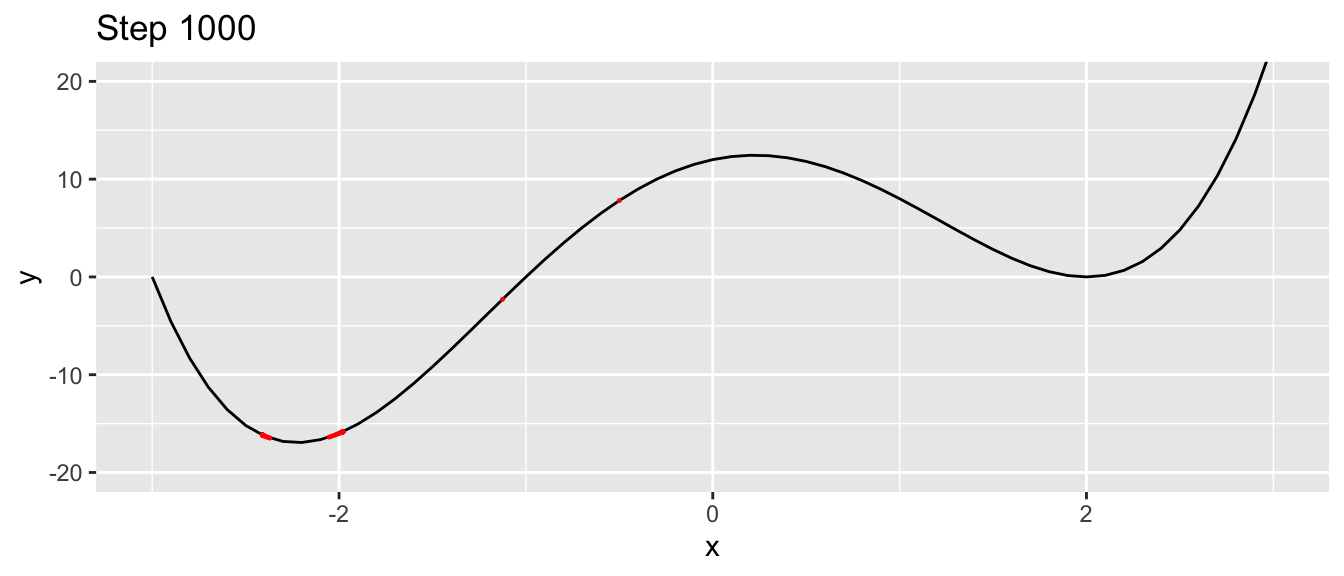

Figure 2.8: At the last step of the iteration process, with another starting value.

We can have a look at what happens iteratively with the following animated graph:

saveGIF({
  
  for(i in c(rep(1,5), 2:14, rep(15, 10))){
    p <- 
      ggplot() +
      geom_line(data = df, aes(x = x, y = y)) +
      geom_point(data = df_plot %>% slice(i), 
                 mapping = aes(x = x_1, y= f(x_1)),
                 colour = "red", size = 2) +
      geom_abline(data = df_plot %>% slice(i),
                  aes(slope = gradient, intercept = intercept),
                  colour = "blue") +
      coord_cartesian(ylim = c(-20, 20)) +
      labs(title = str_c("Step ", i))
    print(p)
  }
  
}, movie.name = "example_single_var_bounce.gif", interval = 0.5, 
ani.width = 720, ani.height = 480)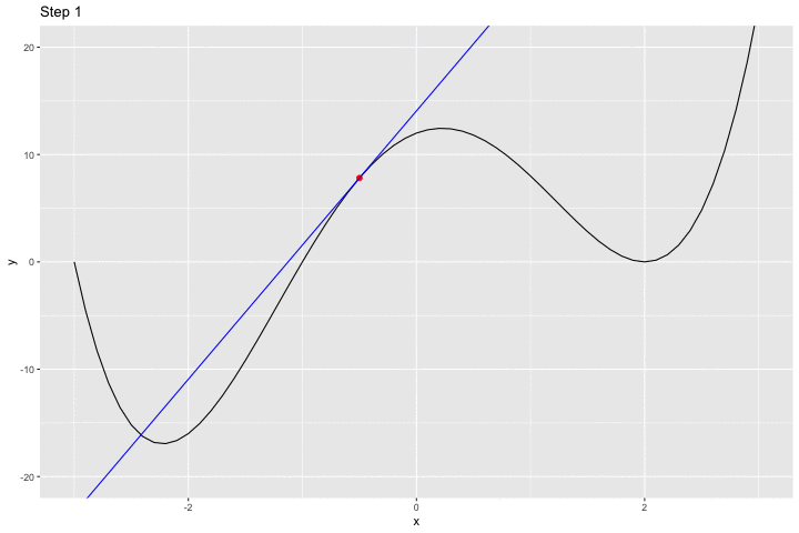

We jumped around the minimum and never reached it.

The algorithm is also sensitive to the starting point.

learning_rate <- 0.01
nb_max_iter <- 1000
tolerance <- 10^-5
# Starting value
x_1 <- .5
# To keep track of the values through the iterations
x_1_values <- x_1
y_1_values <- f(x_1)
gradient_values <- NULL
intercept_values <- NULL

for(i in 1:nb_max_iter){
  # Steepest ascent:
  grad <- grad(func = f, x = c(x_1))
  
  intercept_value <- -grad*x_1 + f(x_1)
  # Keeping track
  gradient_values <- c(gradient_values, grad)
  intercept_values <- c(intercept_values, intercept_value)
  
  # Updating the value
  x_1 <- x_1 - learning_rate * grad
  y_1 <- f(x_1)
  
  # Keeping track
  x_1_values <- c(x_1_values, x_1)
  y_1_values <- c(y_1_values, y_1)
  
  # Stopping if no improvement (decrease of the cost function too small)
  if(abs(y_1_values[i] - y_1) < tolerance) break
  
}

Let us check whether we converged:

## [1] 33

ifelse(i < nb_max_iter,
       "The algorithm converged.",
       "The algorithm did not converge.")

## [1] "The algorithm converged."

Yes. But let us look at where.

df_plot <- 
  tibble(x_1 = x_1_values[-length(x_1_values)],
         y = f(x_1),
         gradient = gradient_values,
         intercept = intercept_values
  )
df_plot

## # A tibble: 33 × 4
##      x_1     y gradient intercept
##    <dbl> <dbl>    <dbl>     <dbl>
##  1 0.5   11.8     -4.50      14.1
##  2 0.545 11.6     -5.16      14.4
##  3 0.597 11.3     -5.89      14.8
##  4 0.656 10.9     -6.67      15.3
##  5 0.722 10.5     -7.49      15.9
##  6 0.797  9.87    -8.32      16.5
##  7 0.880  9.15    -9.12      17.2
##  8 0.972  8.28    -9.82      17.8
##  9 1.07   7.29   -10.4       18.4
## 10 1.17   6.20   -10.7       18.7
## # … with 23 more rows

ggplot() +
  geom_line(data = df, aes(x = x, y = y)) +
  geom_point(data = df_plot, aes(x = x_1, y= f(x_1)), colour = "red") +
  coord_cartesian(ylim = c(-20, 20)) +
  labs(title = str_c("Step ", i))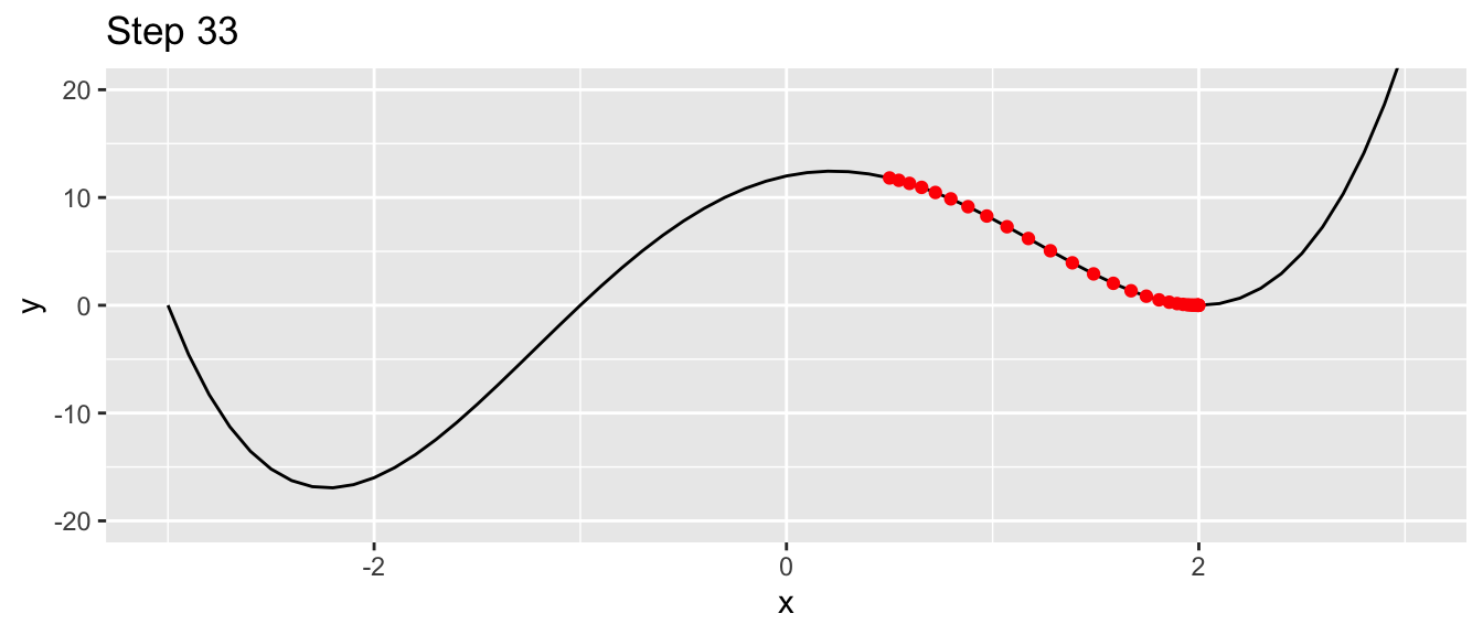

Figure 2.9: Ending up in a local minimum.

This time, we ended up in a local minimum.

Now let us increase the dimension of our problem, and move on to a function defined with two parameters. We will consider more afterwards, but then we will not be able to visualize as easily what happens using graphs.

2.1.3 Moving to Higher Dimensions Optimisation Problems

Let us consider the following data generating process: $f(x_1, x_2) = x_1^2 + x_2^2$.

x_1 <- x_2 <- seq(-2, 2, by = 0.3)
z_f <- function(x_1,x_2) x_1^2+x_2^2
z <- outer(x_1, x_2, z_f)

The representative surface of that function can be visualized as follows:

library(plot3D)
par(mar = c(1, 1, 1, 1))
flip <- 1 # 1 or 2
th = c(-300,120)[flip]
pmat <- 
  persp3D(x = x_1, y = x_2, z = z, colkey=F, contour=T, ticktype = "detailed",
          asp = 1, phi = 30, theta = th, border = "grey10", alpha=.4,
          d = .8,r = 2.8,expand = .6,shade = .2,axes = T,box = T,cex = .1)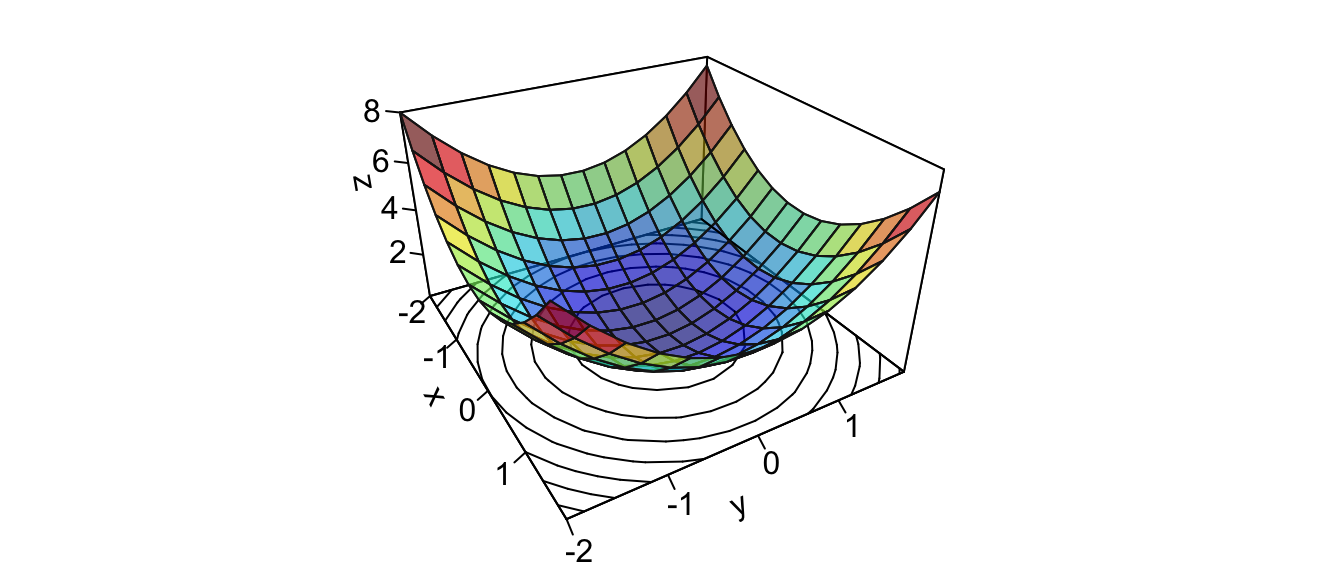

$Surface of a function in $\mathbb{R}^2$.$

Figure 2.10: Surface of a function in $\mathbb{R}^2$.

Once again, we need to initialise the algorithm by picking starting values. Let us pick $\theta = (2,2)$.

theta <- c(x_1 = 1.5, x_2 = 1.5)

Let us look at this point on the graph:

zz <- z_f(theta[["x_1"]], theta[["x_2"]])
new_point <- trans3d(theta[["x_1"]], theta[["x_2"]], zz,
                     pmat = pmat)


par(mar = c(1, 1, 1, 1))
flip <- 1 # 1 or 2
th = c(-300,120)[flip]
pmat <- 
  persp3D(x = x_1, y = x_2, z = z, colkey=F, contour=T, ticktype = "detailed",
          asp = 1, phi = 30, theta = th, border = "grey10", alpha=.4,
          d = .8,r = 2.8,expand = .6,shade = .2,axes = T,box = T,cex = .1)
points(new_point,pch = 20,col = "red", cex=2)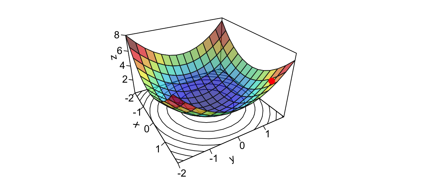

Figure 2.11: Starting point.

From that point, we need to decide the direction to go to and the magnitude of the step to take in that direction. The direction is obtained by computing the first derivative of the objective function $f(\cdot)$ with respect to each argument $x_1$ and $x_2$, at point $\theta$. In other words, we need to evaluate the gradient of the function at point $\theta$.

\[\nabla f(\theta) = \begin{bmatrix}\frac{\partial f}{\partial x_1}(\theta)\\ \frac{\partial f}{\partial x_2}(\theta)\end{bmatrix}\]

The values will give us the steepest ascent. Once the learning rate is decided, we just need to update each argument by moving in the opposite direction of the steepest ascent. The updated value of the parameters after the end of the $t$th step will be as follows:

\[\begin{bmatrix}x_1^{(t+1)} \\ x_2^{(t+1)}\end{bmatrix} = \begin{bmatrix}x_1^{(t)} \\ x_2^{(t)}\end{bmatrix} - \eta \begin{bmatrix}\frac{\partial f}{\partial x_1}(x_1^{(t)}, x_2^{(t)})\\ \frac{\partial f}{\partial x_2}(x_1^{(t)}, x_2^{(t)})\end{bmatrix},\] where $\begin{bmatrix}x_1^{(t+1)} \\ x_2^{(t+1)}\end{bmatrix}$ is the updated vector of parameters, $\begin{bmatrix}x_1^{(t)} \\ x_2^{(t)}\end{bmatrix}$ is the current value of the vector of parameters, $\eta \in \mathbb{R}^+$ is the learning rate, and $\begin{bmatrix}\frac{\partial f}{\partial x_1}(x_1^{(t)}, x_2^{(t)})\\ \frac{\partial f}{\partial x_2}(x_1^{(t)}, x_2^{(t)})\end{bmatrix}$ is the gradient of the function at point $\theta = \left(x_1^{(t)}, x_2^{(t)}\right)$.

In a more general context, when at a point $\mathbf{\theta}\in\mathbb{R}^p$, at any step $t\leq 0$, the gradient descent algorithm tries to move in a direction $\delta \mathbf{\theta}$ such that $\mathcal{L}\left(\mathbf{\theta}^{(t)} + \delta\mathbf{\theta} \right) < \mathcal{L}\left(\mathbf{\theta}^{(t)}\right)$. The choice of $\delta\mathbf{\theta}$ is made such that $\delta\mathbf{\theta} = -\eta \cdot \nabla\mathcal{L}\left(\mathbf{\theta}^{(t)}\right)$:

\[\mathbf{\theta}^{(t+1)} = \mathbf{\theta}^{(t)} -\eta \cdot \nabla\mathcal{L}\left(\mathbf{\theta}^{(t)}\right)\]

Note : the choice of $\delta\mathbf{\theta}$ is made based on the first-order Taylor approximation. If $\mathcal{L} : \mathbb{R}^p \rightarrow \mathbb{R}$ is differentiable at point $\mathbf{\theta}$, for any small change $\delta\mathbf{\theta}$, the best linear approximation to $\mathcal{L}$ is given by:

\[\mathcal{L}(\mathbf{\theta} + \delta\mathbf{\theta}) = \mathcal{L}({\mathbf{\theta}}) + \nabla\mathcal{L}(\mathbf{\theta})^{\top} \delta\mathbf{\theta} + \mathcal{O}(\lVert \delta^2\mathbf{\theta} \rVert)\] We want to get :

\[\nabla\mathcal{L}(\mathbf{\theta})^{\top} \delta\mathbf{\theta} < 0\]

\[\begin{align*} & \mathcal{L}(\mathbf{\theta} + \delta \mathbf{\theta}) < \mathcal{L}(\mathbf{\theta})\\ \Leftrightarrow & \mathcal{L}({\mathbf{\theta}}) + \nabla\mathcal{L}(\mathbf{\theta})^{\top} \delta\mathbf{\theta} < \mathcal{L}({\mathbf{\theta}})\\ \Leftrightarrow &\nabla\mathcal{L}(\mathbf{\theta})^{\top} \delta\mathbf{\theta} < 0. \end{align*}\]

This dot product takes its minimum value when $\delta \mathbf{\theta} = -\nabla\mathcal{L}(\mathbf{\theta})$. This gives the direction to go to. This does not tell us, however, the magnitude of the step that we should take.

Let us rewrite our function $f(\cdot)$ so that we can calculate its gradient by numerical approximation at a given point $\theta$ using grad() from {numDeriv}.

z_f_to_optim <- function(theta){
  x_1 <- theta[["x_1"]]
  x_2 <- theta[["x_2"]]
  x_1^2 + x_2^2
}

Let us set a learning rate:

learning_rate <- 10^-2

The steepest ascent can be obtained as follows:

grad <- grad(func = z_f_to_optim, x = theta)
grad

## [1] 3 3

The values can then be updated:

updated_x_1 <- theta[["x_1"]] - learning_rate * grad[1]
updated_x_2  <- theta[["x_2"]] - learning_rate * grad[2]
updated_theta <- c(x_1 = updated_x_1, x_2 = updated_x_2)
updated_theta

##  x_1  x_2 
## 1.47 1.47

On the graph:

par(mar = c(1, 1, 1, 1))
flip <- 1 # 1 or 2
th = c(-300,120)[flip]
pmat <- 
  persp3D(x = x_1, y = x_2, z = z, colkey=F, contour=T,
          ticktype = "detailed", asp = 1, phi = 30, theta = th,
          border = "grey10", alpha=.4, d = .8,r = 2.8,
          expand = .6,shade = .2,axes = T,box = T,cex = .1)
updated_zz <- z_f(updated_theta[["x_1"]], updated_theta[["x_2"]])
new_point_2 <- trans3d(updated_theta[["x_1"]],
                       updated_theta[["x_2"]],
                       updated_zz,
                       pmat = pmat)
points(new_point,pch = 20,col = "red", cex=2)
points(new_point_2,pch = 20,col = "darkgreen", cex=2)

Figure 2.12: Updated value after the first iteration.

Then, we need to repeat the updating process. The full algorithm can be written this way:

learning_rate <- 10^-1
nb_max_iter <- 100
tolerance <- 10^-5

# Starting values
theta <- c(x_1 = 1.5, x_2 = 1.5)

# To keep track of what happens at each iteration
theta_values <- list(theta)
y_values <- z_f_to_optim(theta)

for(i in 1:nb_max_iter){
  # Steepest ascent
  grad <- grad(func = z_f_to_optim, x = theta)
  
  # Updating the parameters
  updated_x_1 <- theta[["x_1"]] - learning_rate * grad[1]
  updated_x_2  <- theta[["x_2"]] - learning_rate * grad[2]
  theta <- c(x_1 = updated_x_1, x_2 = updated_x_2)
  
  # Keeping track
  theta_values <- c(theta_values, list(theta))
  
  # Checking for improvement
  y_updated <- z_f_to_optim(theta)
  y_values <- c(y_values, y_updated)
  if(abs(y_values[i] - y_updated) < tolerance) break
  
}

Let us check at which iteration the algorithm stopped:

## [1] 28

ifelse(i < nb_max_iter,
       "The algorithm converged.",
       "The algorithm did not converge.")

## [1] "The algorithm converged."

Graphically:

par(mar = c(1, 1, 1, 1))
flip <- 1 # 1 or 2
th = c(-300,120)[flip]
pmat <- 
  persp3D(x = x_1, y = x_2, z = z, colkey=F, contour=T, 
          ticktype = "detailed", asp = 1, phi = 30, theta = th, 
          border = "grey10", alpha=.4, d = .8,r = 2.8,
          expand = .6,shade = .2,axes = T,box = T,cex = .1)

xx <- map_dbl(theta_values, "x_1")
yy <- map_dbl(theta_values, "x_2")
zz <- y_values
new_point <- trans3d(xx,yy,zz,pmat = pmat)
lines(new_point,pch = 20,col = "red", cex=2, lwd=2)
points(new_point,pch = 20,col = "red", cex=2)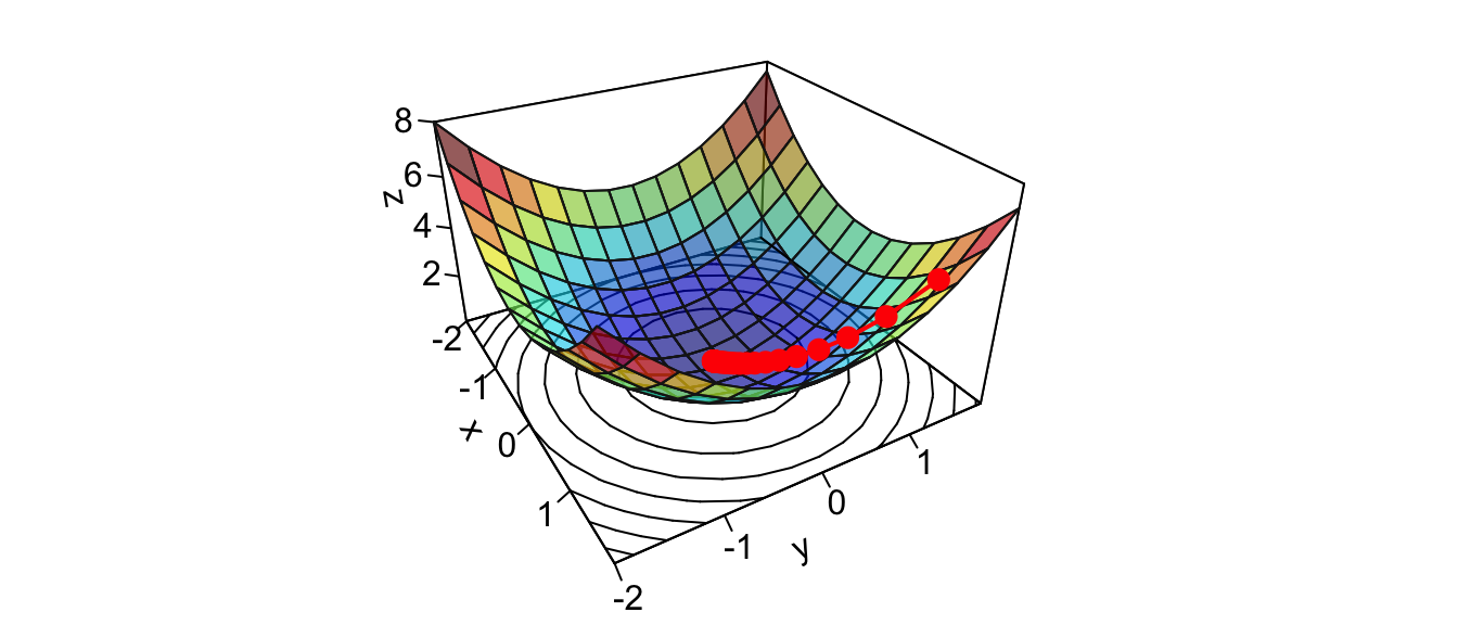

Figure 2.13: At the end of the iterative process.

To have a look, step by step:

library(animation)
saveGIF({
  
  for(j in c(rep(1,5), 2:(i-1), rep(i, 10))){
    
    par(mar = c(1, 1, 1, 1))
    flip <- 1 # 1 or 2
    th = c(-300,120)[flip]
    pmat <- 
      persp3D(x = x_1, y = x_2, z = z, colkey=F, contour=T, 
              ticktype = "detailed", asp = 1, phi = 30, theta = th,
              border = "grey10", alpha=.4, d = .8,r = 2.8,
              expand = .6,shade = .2,axes = T,box = T,cex = .1)
    
    xx <- map_dbl(theta_values, "x_1")[1:j]
    yy <- map_dbl(theta_values, "x_2")[1:j]
    zz <- y_values[1:j]
    new_point <- trans3d(xx,yy,zz,pmat = pmat)
    lines(new_point,pch = 20,col = "red", cex=2, lwd=2)
    points(new_point,pch = 20,col = "red", cex=2)
  }
  
}, movie.name = "descent_2D_sphere.gif", interval = 0.01,
ani.width = 720, ani.height = 480)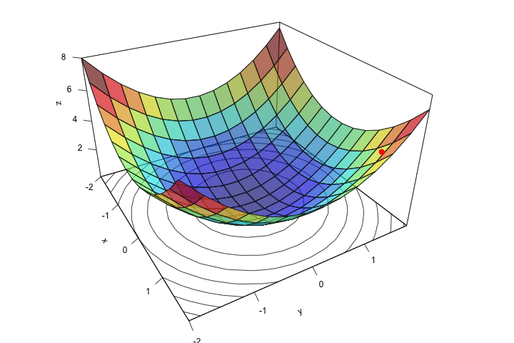

Figure 2.14: Descent, step by step.

With this example, we quickly converged to a solution. But the surface can be a bit more complex. Let us consider another data generating process, Mishra’s Bird function:

\[f(x_1, x_2) = \sin(x_2) * \exp(1-\cos(x_1))^2 + \cos(x_1) * \exp(1-\sin(x_2))^2 + (x_1-x_2)^2.\]

First, let us generate some data:

x_1 <- seq(-6.5, 0, by = 0.3)
x_2 <- seq(-10, 0, by = 0.3)
z_f <- function(x_1,x_2){
  sin(x_2)*exp(1-cos(x_1))^2 + cos(x_1)*exp(1-sin(x_2))^2 + (x_1-x_2)^2
}
z <- outer(x_1, x_2, z_f)

A graphical representation of the surface:

par(mar = c(1, 1, 1, 1))
flip <- 2 # 1 or 2
theta = c(-300,120)[flip]
pmat <- 
  persp3D(x = x_1, y = x_2, z = z, colkey=F, contour=T, 
          ticktype = "detailed", asp = 1, phi = 30, theta = th, 
          border = "grey10", alpha=.4, d = .8,r = 2.8,
          expand = .6,shade = .2,axes = T,box = T,cex = .1)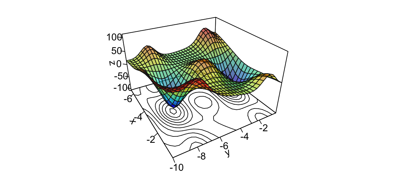

$A more complex function in $\mathbb{R}^2$.$

Figure 2.15: A more complex function in $\mathbb{R}^2$.

The function that needs to be optimized need to be rewritten so that the first argument is the vector of parameters over which minimisation is to take place.

z_f_to_optim <- function(theta){
  x_1 <- theta[1]
  x_2 <- theta[2]
  sin(x_2) * exp(1-cos(x_1))^2 + cos(x_1) * exp(1-sin(x_2))^2 + 
    (x_1-x_2)^2
}

Let us create a function that uses the gradient descent algorithm to try find the minimum.

#' @param par Initial values for the parameters to be optimized over.
#' @param fn A function to be minimized, with first argument the vector 
#'           of parameters over which minimisation is to take place.
#'           It should return a scalar result.
#' @param learning_rate Learning rate.
#' @param nb_max_iter The maximum number of iterations (default to 100).
#' @param tolerance The absolute convergence tolerance (default to 10^-5).
gradient_descent <- function(par, fn, learning_rate, 
                             nb_max_iter = 100, tolerance = 10^-5){
  
  # To keep track of what happens at each iteration
  par_values <- list(par)
  y_values <- fn(par)
  
  for(i in 1:nb_max_iter){
    # Steepest ascent
    grad <- grad(func = fn, x = par)
    
    # Updating the parameters
    par <- par - learning_rate * grad
    
    # Keeping track
    par_values <- c(par_values, list(par))
    
    # Checking for improvement
    y_updated <- fn(par)
    y_values <- c(y_values, y_updated)
    rel_diff <- abs(y_values[i] - y_updated)
    if(rel_diff < tolerance) break
    
  }
  
  # Has the algorithm converged?
  convergence <- i < nb_max_iter | (rel_diff < tolerance)
  
  structure(
    list(
      par = par,
      value = y_updated,
      pars = do.call("rbind", par_values),
      values = y_values,
      convergence = convergence,
      nb_iter = i,
      nb_max_iter = nb_max_iter,
      tolerance = tolerance
    ))
  
}

Now this optimisation function can be called. Let us start at $\theta = (-6,-2)$, and try to find the minimum with a learning rate of $10^{-2}$ over at most 100 iterations.

res_optim <- 
  gradient_descent(par = c(-6, -2), fn = z_f_to_optim,
                   learning_rate = 10^-2,
                   nb_max_iter = 100,
                   tolerance = 10^-5)

Let us check whether the algorithm converged:

res_optim$convergence

## [1] TRUE

res_optim$nb_iter

## [1] 41

The algorithm has converged. Let us look at the point we ended up with:

res_optim$par

## [1] -3.122755 -1.589316

res_optim$value

## [1] -106.7877

And graphically:

par(mar = c(1, 1, 1, 1))
pmat <- 
  persp3D(x = x_1, y = x_2, z = z, colkey=F, contour=T, 
          ticktype = "detailed", asp = 1, phi = 30, theta = 120, 
          border = "grey10", alpha=.4, d = .8,r = 2.8,
          expand = .6,shade = .2,axes = T,box = T,cex = .1)

xx <- res_optim$pars[,1]
yy <- res_optim$pars[,2]
zz <- res_optim$values
new_point <- trans3d(xx,yy,zz,pmat = pmat)
lines(new_point,pch = 20,col = "red", cex=2, lwd=2)
points(new_point,pch = 20,col = "red", cex=2)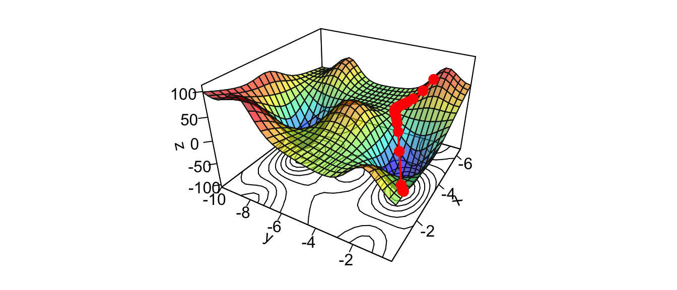

Figure 2.16: Interative process We end up in a local minimum.

saveGIF({
  for(j in c(rep(1,5), 2:(res_optim$nb_iter-1), rep(res_optim$nb_iter, 10))){
    
    par(mar = c(1, 1, 1, 1))
    pmat <- 
      persp3D(x = x_1, y = x_2, z = z, colkey=F, contour=T, 
              ticktype = "detailed", asp = 1, phi = 30, theta = 120, 
              border = "grey10", alpha=.4, d = .8,r = 2.8,
              expand = .6, shade = .2,axes = T,box = T,cex = .1,
              main = str_c("Step ", j))
    
    xx <- res_optim$pars[1:j,1]
    yy <- res_optim$pars[1:j,2]
    zz <- res_optim$values[1:j]
    new_point <- trans3d(xx,yy,zz,pmat = pmat)
    lines(new_point,pch = 20,col = "red", cex=2, lwd=2)
    points(new_point,pch = 20,col = "red", cex=2)
  }
  
}, movie.name = "descent_3D_Mishra.gif", interval = 0.01, 
ani.width = 720, ani.height = 480)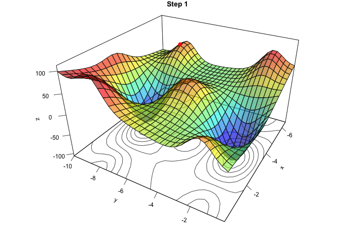

Figure 2.17: Starting from another initial value, we end-up in another local minimum.

We ended up in the minimum.

Another way to look at the gradient descent is through the following contour plot. At each iteration, we decide in which direction to go:

d <- tibble(x = res_optim$pars[,1],
            y = res_optim$pars[,2],
            z = res_optim$values)
contour2D(x=x_1, y=x_2, z=z, colkey=F, main="Contour plot",
          xlab="x_1", ylab="x_2")
points(x=d$x, y=d$y, t="p", pch=19, col = "red")
for(k in 2:(nrow(d+1))) 
  segments(x0 = d$x[k-1], y0 = d$y[k-1], 
           x1 = d$x[k], y1 = d$y[k], col= 'red')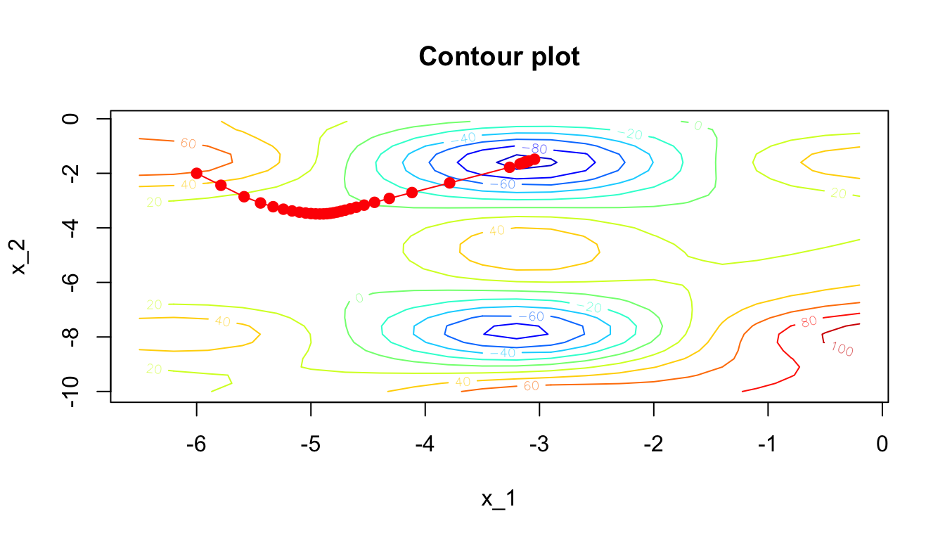

Figure 2.18: Another grapghical representation: contour plot.

Let us change the starting point to begin with $\theta = (-6,-4)$ (let us also increase the maximum number of iterations).

res_optim <- 
  gradient_descent(par = c(-6, -4), fn = z_f_to_optim,
                   learning_rate = 10^-2,
                   nb_max_iter = 1000,
                   tolerance = 10^-5)

Let us check whether the algorithm converged:

res_optim$convergence

## [1] TRUE

res_optim$nb_iter

## [1] 141

The algorithm has also converged. Let us look at the point we ended up with:

par(mar = c(1, 1, 1, 1))
pmat <- 
  persp3D(x = x_1, y = x_2, z = z, colkey=F, contour=T, 
          ticktype = "detailed", asp = 1, phi = 30, theta = 120,
          border = "grey10", alpha=.4, d = .8,r = 2.8,
          expand = .6, shade = .2,axes = T,box = T,cex = .1)

xx <- res_optim$pars[,1]
yy <- res_optim$pars[,2]
zz <- res_optim$values
new_point <- trans3d(xx,yy,zz,pmat = pmat)
lines(new_point,pch = 20,col = "red", cex=2, lwd=2)
points(new_point,pch = 20,col = "red", cex=2)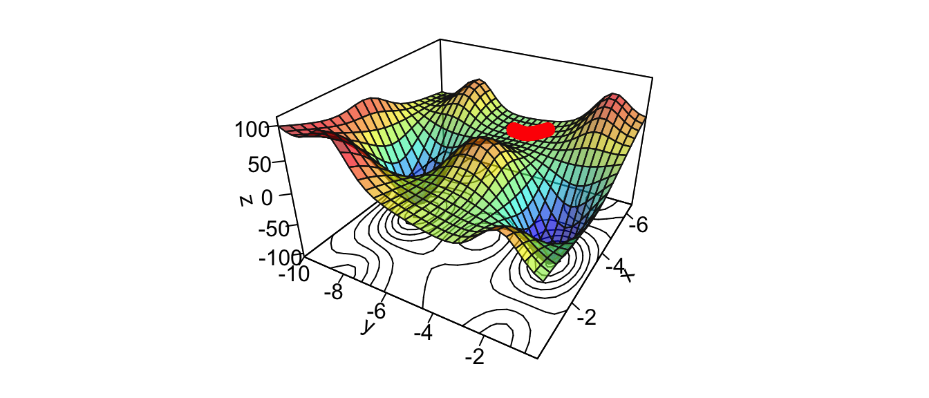

Figure 2.19: Getting stuck in a plateau.

We reached a local minimum.

d <- tibble(x = res_optim$pars[,1],
            y = res_optim$pars[,2],
            z = res_optim$values)
contour2D(x=x_1, y=x_2, z=z, colkey=F, main="Contour plot", 
          xlab="x_1", ylab="x_2")
points(x=d$x, y=d$y, t="p", pch=19, col = "red")
for(k in 2:(nrow(d+1))) 
  segments(x0 = d$x[k-1], y0 = d$y[k-1], x1 = d$x[k],
           y1 = d$y[k], col= 'red')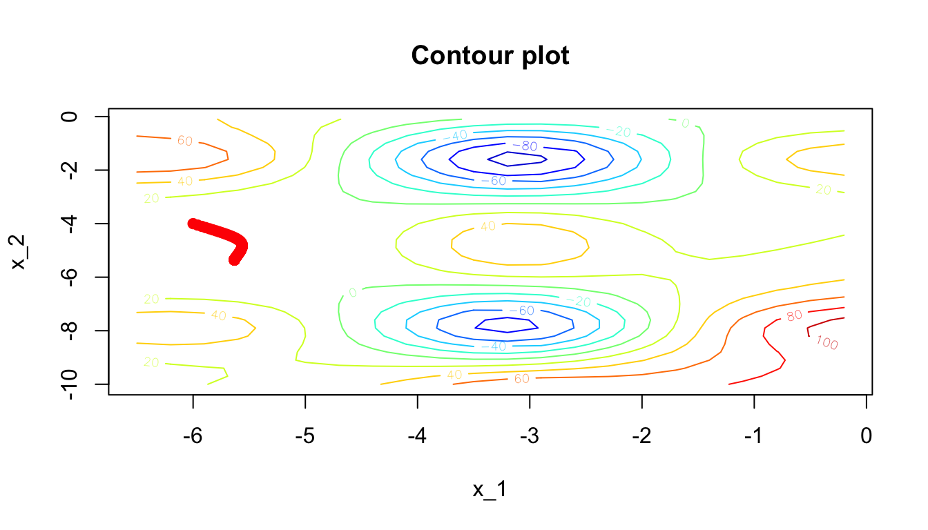

Figure 2.20: Contour plot: getting stuck in a plateau.

2.1.4 Case Study: Linear Regression

Let us generate some data.

\[y_i = 3x_i - 2 + \varepsilon_i, \quad i=1,\ldots,n,\] where $\varepsilon$ is normally distributed with zero mean and variance $\sigma^2=4$.

set.seed(123)
# Number of observations
n <- 50
# x randomly drawn from a continuous uniform distribution with bounds [0,10]
x <- runif(min = 0, max = 10, n = n)
# Error term from Normal distribution with zero mean and variance 4
error <- rnorm(n = n, mean = 0, sd = 2)
# Response variable
beta_0 <- 3
beta_1 <- -2
y <- beta_0*x + beta_1 + error

Let us put the data in a table:

df <- tibble(x = x, y = y)
df

## # A tibble: 50 × 2
##        x      y
##    <dbl>  <dbl>
##  1 2.88   3.25 
##  2 7.88  23.3  
##  3 4.09  10.6  
##  4 8.83  22.2  
##  5 9.40  28.7  
##  6 0.456  0.220
##  7 5.28  13.3  
##  8 8.92  26.6  
##  9 5.51  16.3  
## 10 4.57  13.3  
## # … with 40 more rows

ggplot(data = df, aes(x = x, y = y)) + geom_point() +
  geom_abline(slope = 3, intercept = -2) +
  labs(title = "y = f(x)")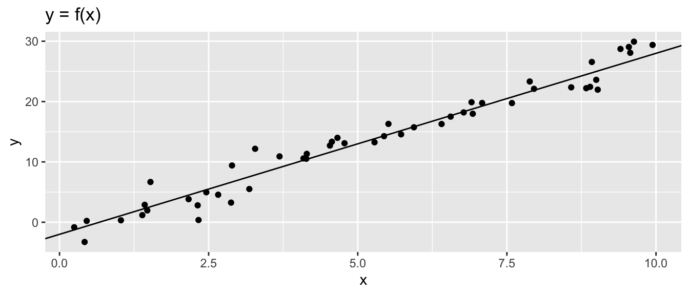

Figure 2.21: Data Generating Process and synthetic data.

Now, let us suppose that we do not know anymore the parameters $\beta_0$ and $\beta_1$. The only things we assume are that there exists a linear relationship between $y$ and $x$ and that the error term is normally distributed with zero mean and (unknown) variance $\sigma^2$.

In other words, we would like to estimate the following model:

\[y_i = \beta_0 + \beta_1x_i + \varepsilon_i, \quad i=1,\ldots,n,\]

where $\varepsilon ~\mathcal{N}(0, \sigma^2)$, and where $\beta_0$, $\beta_1$ (and $\sigma^2$) are unknown and need to be estimated.

We would like to obtain estimates of $\beta_0$ and $\beta_1$ such that the loss function (our objective function) is the smallest. The loss function we will use is the mean squared error:

\[\mathcal{L}(\beta) = \frac{1}{n}\sum_{i=1}^n \left( y_i - \hat{y}_i) \right)^2,\]

where $\hat{y}_i = \hat{\beta_0} + \hat{\beta_1}x_i$, and where $\hat{\beta_0}$ and $\hat{\beta_1}$ are the estimates of $\beta_0$ and $\beta_1$, respectively.

We will use the gradient descent algorithm to estimate these parameters so as to minimise this loss function.

The function to optimise:

obj_function <- function(theta, y){
  y_pred <- theta[1] + theta[2]*x
  mean((y - y_pred)^2)
}

We need some starting values for $\beta_0$ and $\beta_1$:

beta <- c(0, 0)

Let us keep track of the updated values throughout the iterations:

beta_values <- beta
mse_values  <- NULL

We need to pick a learning rate:

learning_rate <- 10^-2

Let us set a maximum number of iterations:

nb_max_iter <- 1000

And an absolute tolerance:

abstol <- 10^-5

for(i in 1:nb_max_iter){
  # Predctions with the current values:
  y_pred <- beta[1] + beta[2]*x
  
  # Just for keeping track
  mse <- mean((y - y_pred)^2)
  mse_values <- c(mse_values, mse)
  
  gradient <- grad(func = obj_function, x = beta, y=y)
  
  # We could also use the exact expression here:
  # deriv_loss_beta <- -2/n * sum( y - y_pred )
  # deriv_loss_beta_0 <- -2/n * sum( x*(y - y_pred) )
  
  
  # Updating the value
  beta <- beta - learning_rate * gradient
  
  # Keeping track of the changes
  beta_values <- rbind(beta_values, beta)
  
  
  if(i>1){
    rel_diff <- abs(mse_values[i] - mse_values[i-1])
    if(rel_diff < abstol) break
  }
  
}

Has the algorithm converged?

print(str_c("Number of iterations: ", i))

## [1] "Number of iterations: 790"

convergence <- i < nb_max_iter | (rel_diff < abstol)
convergence

## [1] TRUE

The estimated values:

beta

## [1] -2.218623  3.066613

For comparison, the OLS estimates are as follows:

lm(y~x)

## 
## Call:
## lm(formula = y ~ x)
## 
## Coefficients:
## (Intercept)            x  
##      -2.285        3.076

We can notice that the MSE quickly converges to the variance of the error:

ggplot(data = tibble(mse = mse_values) %>% 
         mutate(iteration = row_number()) %>% 
         filter(iteration > 1),
       aes(x = iteration, y = mse)) +
  geom_line()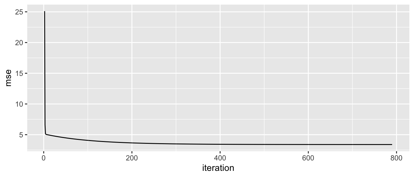

Figure 2.22: Quick convergence of the MSE to the variance of the error.

We can have a look at the updates throughout the iterative process:

as_tibble(beta_values, .name_repair = "minimal") %>% 
  magrittr::set_colnames(c("beta_0", "beta_1")) %>% 
  mutate(iteration = row_number()) %>% 
  ggplot(data = ., aes(x = beta_0, y = beta_1)) +
  geom_point(aes(colour = iteration), size = .1)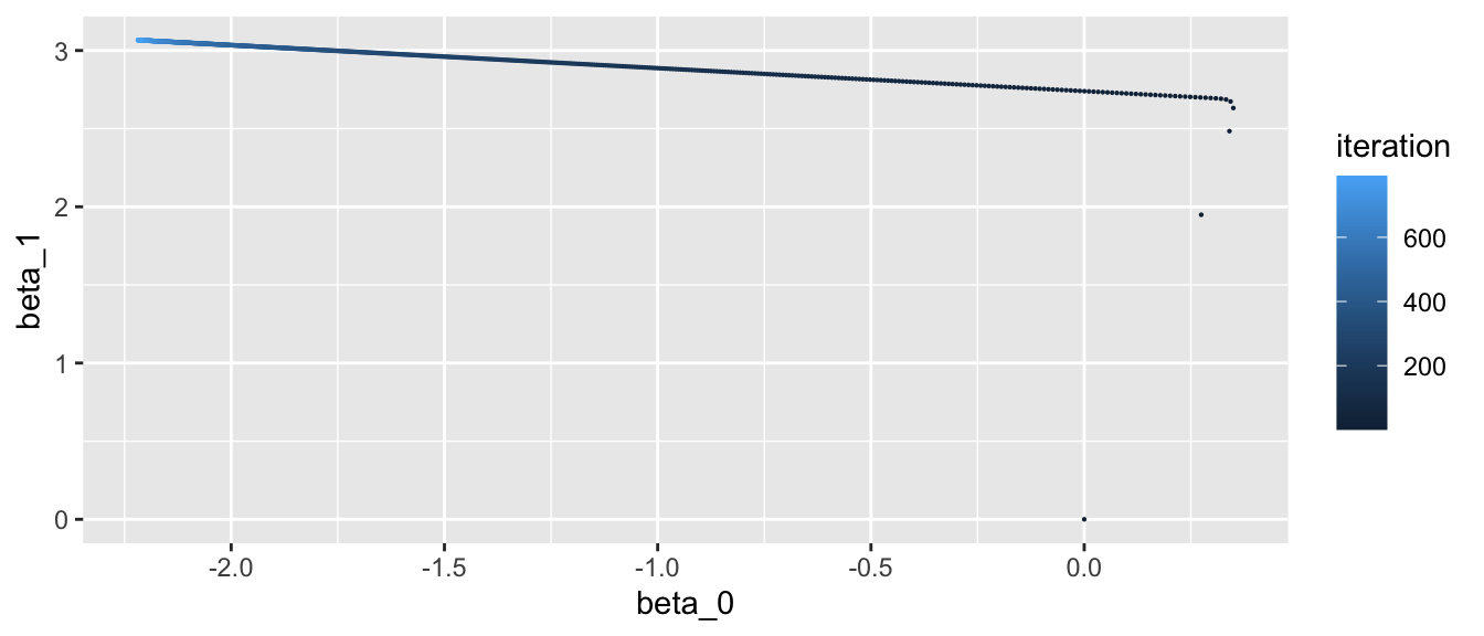

Figure 2.23: Updated values at each iteration.

2.2 Variants of the Gradient Descent Algorithm

So far, we have estimated the $p$ parameters that minimise an objective function $\mathcal{L}(\theta)$, where $\theta$ is a vector of the $p$ parameters to be estimated.

We have seen that the gradient descent algorithm updates the value of the $i$th parameter using the following rule: \[\theta^{(t+1)} = \theta^{(t)} - \eta \cdot \nabla \mathcal{L}\big(\theta^{(t)}\big)\]

In the previous example, to compute the gradient of the objective function $\mathcal{L}$, we have used the whole dataset. The learning rate $eta$ was a constant. In this section, we will consider different ways of updating the parameters. First, we will focus on the frequency of updates and on the samples used to update the parameters. Then, we will have a glance at ways used to make the learning rate vary along the iteration process.

Before jumping to those aspects, let us sum up how the gradient descent algorithm works:

Gradient Descent Algorithm

Randomly pick starting values for the parameters
Compute the gradient of the objective function at the current value of the parameters using all the observations from the training sample
Update the parameters
Repeat from step 2 until a fixed number of iteration or until convergence.

2.2.1 Frequency of Updates & Samples Used

2.2.1.1 Stochastic Gradient Descent

Actually, multiple ways can be used to compute the gradient of the objective function. Instead of updating the parameters using all the observations, the former can be updated using a single observation from the dataset at each iteration. Each sample observation is used in turn to evaluate the objective function and to update the parameters. Once all the observations have been used to update the parameters, we say that we have passed an epoch. The overall procedure in which a single observation (as opposed to the whole dataset) is used to update the parameters is called Stochastic Gradient Descent (SGD).

As opposed to Gradient Descent, Stochastic Gradient Descent do not require to train over the entire dataset, which may not be feasible depending on the size of the data at hand, or may be very slow. Imagine having a large dataset with a high number of features $p$ and a large number of observations $N$. At each iteration, with Gradient Descent, we need to compute $p$ first-order derivative for $N$ observations. With Stochastic Gradient Descent, instead of computing the first-order derivative for all $N$ observations, a single randomly drawn observation is used. The iteration is thus faster with Stochastic Gradient Descent. However, the update process becomes noisier and the algorithm converges at a lower rate. But the fact that the update process becomes noisier may not be a curse: it can allow us to avoid ending up in a local minimum.

As the update of the parameters is done for each observation, it is not possible to rely on vectorized or parallel implementation of this process.

To sum up, the algorithm works as follows:

Stochastic Gradient Descent Algorithm

Randomly pick starting values for the parameters
Select an observation
Compute the gradient of the objective function using the observation from step 2
Update the parameters
Repeat from step 2 until all the observations from the training sample have been used: this constitutes an epoch
Repeat the procedure from 2 to 5 to complete multiple epochs.

At iteration $t$, the parameters are updated using the $i$th observation:

\[\theta^{(t+1)} = \theta_i^{(t)} - \eta \cdot \nabla \mathcal{L}\big(\theta^{(t)} ; X_i\big)\]

Let us apply this algorithm to estimate the parameters of a linear model. We can generate 1000 observations from the following process: \[y_i = \beta_0 + \beta_{1} x_{1,i} + \beta_{2} x_{2,i} + \varepsilon_i, \quad i=1,\ldots,N\] where $x_1$ and $x_2$ are randomly drawn from a $\mathcal{U}(0,10)$ distribution and $\varepsilon \sim \mathcal{N}(0,2)$.

Let us generate some data:

set.seed(123)
# Number of observations
n <- 1000
# x randomly drawn from a continuous uniform distribution with bounds [0,10]
x_1 <- runif(min = 0, max = 10, n = n)
x_2 <- runif(min = 0, max = 10, n = n)
# Error term from Normal distribution with zero mean and variance 4
error <- rnorm(n = n, mean = 0, sd = 2)
# Response variable
beta_0 <- 3
beta_1 <- -2
beta_2 <- .5
true_beta <- c(beta_0=beta_0, beta_1=beta_1, beta_2=beta_2)
y <- beta_0 + beta_1*x_1 + beta_2*x_2 + error

The objective function is the Mean Squared Error:

obj_function <- function(theta, y, X){
  y_pred <- X%*%theta
  mean((y - y_pred)^2)
}

We can construct the matrix of predictors as follows:

X <- cbind(rep(1, n), x_1, x_2)
colnames(X) <- c("Intercept", "x_1", "x_2")
head(X)

##      Intercept      x_1      x_2
## [1,]         1 2.875775 2.736227
## [2,]         1 7.883051 5.938669
## [3,]         1 4.089769 1.601848
## [4,]         1 8.830174 8.534302
## [5,]         1 9.404673 8.477392
## [6,]         1 0.455565 4.778868

We need some initial values for the vector of parameters:

beta <- c(1,1,1)

We can set the learning rate to $10^-2$. We will only consider 10 epochs here,

learning_rate <- 10^-2
nb_epoch <- 20

To keep track of the process:

mse_values  <- NULL

We will compute the MSE after each epoch, on the whole dataset.

# pb <- txtProgressBar(min = 1, max=nb_epoch, style=3)
for(i_epoch in 1:nb_epoch){
  cat("\n----------\nEpoch: ", i_epoch, "\n")
  
  # Shuffle the order of observations
  index <- sample(1:n, size = n, replace=TRUE)
  
  for(i in 1:n){
    # The gradient is estimated using a single observation: the ith
    gradient <- grad(func = obj_function, x=beta,
                     y=y[index[i]], X = X[index[i],])
    # Updating the value
    beta <- beta - learning_rate * gradient
  }
  
  # Just for keeping track (not necessary to run the algorithm)
  # (Significantly slows down the algorithm)
  cost <- obj_function(beta, y, X)
  cat("MSE : ", cost, "\n")
  mse_values <- c(mse_values, cost)
  # End of keeping track
  
  
  # setTxtProgressBar(pb, i_epoch)
}

## 
## ----------
## Epoch:  1 
## MSE :  60.61677 
## 
## ----------
## Epoch:  2 
## MSE :  14.27008 
## 
## ----------
## Epoch:  3 
## MSE :  21.85282 
## 
## ----------
## Epoch:  4 
## MSE :  4.317547 
## 
## ----------
## Epoch:  5 
## MSE :  12.04292 
## 
## ----------
## Epoch:  6 
## MSE :  7.704181 
## 
## ----------
## Epoch:  7 
## MSE :  16.23794 
## 
## ----------
## Epoch:  8 
## MSE :  6.016237 
## 
## ----------
## Epoch:  9 
## MSE :  28.43145 
## 
## ----------
## Epoch:  10 
## MSE :  10.1408 
## 
## ----------
## Epoch:  11 
## MSE :  5.436552 
## 
## ----------
## Epoch:  12 
## MSE :  8.876291 
## 
## ----------
## Epoch:  13 
## MSE :  144.3951 
## 
## ----------
## Epoch:  14 
## MSE :  7.522555 
## 
## ----------
## Epoch:  15 
## MSE :  26.61209 
## 
## ----------
## Epoch:  16 
## MSE :  5.29168 
## 
## ----------
## Epoch:  17 
## MSE :  57.37272 
## 
## ----------
## Epoch:  18 
## MSE :  4.390237 
## 
## ----------
## Epoch:  19 
## MSE :  11.97248 
## 
## ----------
## Epoch:  20 
## MSE :  5.225995

Here are the estimated parameters:

# True values:
true_beta

## beta_0 beta_1 beta_2 
##    3.0   -2.0    0.5

# Estimates values:
(beta_sgd <- beta)

## [1]  2.6187446 -2.1165051  0.8039565

Looking at the MSE value at each epoch:

ggplot(data = tibble(epoch = 1:length(mse_values),
                     MSE = mse_values)) +
  geom_line(mapping = aes(x = epoch, y = MSE))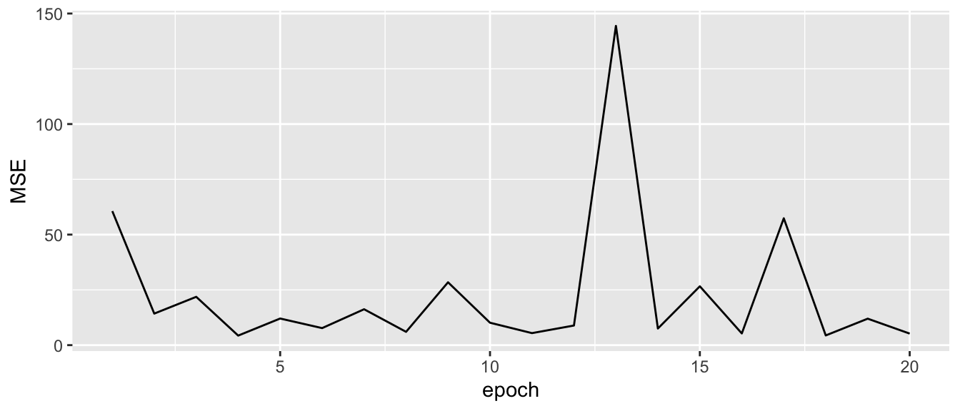

Figure 2.24: Singular Gradient Descent.

We can see that the MSE quickly falls but does not smoothly decreases with the epochs.

Let us create, for convenience, a simple function that performs the Stochastic Gradient Descent for a linear model:

#' Performs Stochastic Gradient Descent for a Linear Model.
#' @param par Initial values for the parameters.
#' @param fn A function to be minimized, with first argument the vector of 
#'           parameters over which minimisation is to take place.
#'           It should return a scalar result.
#' @param y Target variable.
#' @param X Matrix of predictors.
#' @param learning_rate Learning rate.
#' @param nb_epoch Number of epochs.
#' @param silent If TRUE (default), progress information
#'               not printed in the console.
f_sgd <- function(par, fn, y, X, learning_rate=10^-2, nb_epoch=10, silent=TRUE){
  mse_values <- NULL
  for(i_epoch in 1:nb_epoch){
    if(!silent) cat("\n----------\nEpoch: ", i_epoch, "\n")
    n <- nrow(X)
    index <- sample(1:n, size = n, replace=TRUE)
    for(i in 1:n){
      gradient <- grad(func = fn, x=par, y=y[index[i]], X = X[index[i],])
      # Updating the value
      par <- par - learning_rate * gradient
    }
    
    # Just for keeping track (not necessary to run the algorithm)
    # Significantly slows down the algorith
    cost <- fn(par, y, X)
    if(!silent) cat("MSE : ", cost, "\n")
    mse_values <- c(mse_values, cost)
    # End of keeping track
  }
  structure(list(par = par, mse_values = mse_values,
                 nb_epoch = nb_epoch,
                 learning_rate = learning_rate))
}

It can then be applied as follows:

start_time_sgd <- Sys.time()
estim_sgd <- f_sgd(par = c(1,1,1), fn = obj_function, y = y, X = X, 
                   silent=TRUE, nb_epoch = 20)
end_time_sgd <- Sys.time()

The time that elapsed to run through the 20 epochs:

# Time elapsed
end_time_sgd-start_time_sgd

## Time difference of 22.12997 secs

estim_sgd

## $par
## [1]  3.3837401 -1.4333884  0.5377486
## 
## $mse_values
##  [1] 26.254430 20.623584  5.261876 14.536654  5.021757 36.114059 15.058143
##  [8]  7.031129 19.488286  5.029290 21.690363 17.232837 14.928142  9.019636
## [15] 17.868784  6.077928 16.709309 16.596630 11.279380 17.557011
## 
## $nb_epoch
## [1] 20
## 
## $learning_rate
## [1] 0.01

2.2.1.2 Batch Gradient Descent

Another variant of the Gradient Descent algorithm is the Batch Gradient Descent. Again, the gradient of the objective function is computed separately for each observation rather than on the whole dataset. In contrast with what is done with Stochastic Gradient Descent, the parameters are not updated after each observation. The average of the gradients computed for each observation is used to update the parameters only once at each epoch.

As there are fewer updates with this solution than with Stochastic Gradient Descent, the update process is less computationally expensive and less subject to noise. While a less noisy learning process can lead to more stable solutions, they also increase the risk of landing in a local minimum.

To sum up, the algorithm works as follows:

Batch Gradient Descent Algorithm

Randomly pick starting values for the parameters
For each observation, compute the gradient of the objective function
Compute the mean of the gradients computed in step 2
Update the parameters with the mean gradient from step 3
Repeat from step 2 a given number of times.

At iteration $t$, the parameters are updated as follows:

\[\theta^{(t+1)} = \theta^{(t)} - \eta \cdot \frac{1}{n} \sum_{i=1}^{n}\nabla \mathcal{L}\big(\theta^{(t)} ; X_i\big),\]

where $n$ is the size of the training sample.

Let us use the same data as earlier, and use this time the Batch Gradient algorithm instead of the Stochastic Gradient algorithm.

We need starting values for the parameters:

beta <- c(1,1,1)

The learning rate and the number of epochs are the same:

learning_rate <- 10^-2
nb_epoch <- 20

And let us keep track of the MSE through the epochs:

mse_values  <- NULL

# pb <- txtProgressBar(min = 1, max=nb_epoch, style=3)
for(i_epoch in 1:nb_epoch){
  cat("\n----------\nEpoch: ", i_epoch, "\n")
  # For each observation, we need to compute the gradient
  gradients <- rep(0, ncol(X))
  for(i in 1:n){
    gradient_current <- grad(func = obj_function, x=beta, y=y[i], X = X[i,])
    gradients <- gradients+gradient_current
  }
  # Then we divide by the number of observations to get the average
  avg_gradients <- gradients/n
  
  # Updating the value
  beta <- beta - learning_rate * avg_gradients
  
  # Just for keeping track (not necessary to run the algorithm)
  # Significantly slows down the algorith
  cost <- obj_function(beta, y, X)
  cat("MSE : ", cost, "\n")
  mse_values <- c(mse_values, cost)
  # End of keeping track
  
  
  # setTxtProgressBar(pb, i_epoch)
}

## 
## ----------
## Epoch:  1 
## MSE :  30.67738 
## 
## ----------
## Epoch:  2 
## MSE :  17.55995 
## 
## ----------
## Epoch:  3 
## MSE :  13.37346 
## 
## ----------
## Epoch:  4 
## MSE :  10.64122 
## 
## ----------
## Epoch:  5 
## MSE :  8.778509 
## 
## ----------
## Epoch:  6 
## MSE :  7.506044 
## 
## ----------
## Epoch:  7 
## MSE :  6.636364 
## 
## ----------
## Epoch:  8 
## MSE :  6.041603 
## 
## ----------
## Epoch:  9 
## MSE :  5.634493 
## 
## ----------
## Epoch:  10 
## MSE :  5.355469 
## 
## ----------
## Epoch:  11 
## MSE :  5.163874 
## 
## ----------
## Epoch:  12 
## MSE :  5.03196 
## 
## ----------
## Epoch:  13 
## MSE :  4.940786 
## 
## ----------
## Epoch:  14 
## MSE :  4.877425 
## 
## ----------
## Epoch:  15 
## MSE :  4.833054 
## 
## ----------
## Epoch:  16 
## MSE :  4.80165 
## 
## ----------
## Epoch:  17 
## MSE :  4.779102 
## 
## ----------
## Epoch:  18 
## MSE :  4.762605 
## 
## ----------
## Epoch:  19 
## MSE :  4.750244 
## 
## ----------
## Epoch:  20 
## MSE :  4.740712

The estimated values:

# True values:
true_beta

## beta_0 beta_1 beta_2 
##    3.0   -2.0    0.5

# Estimated values:
(beta_batch <- beta)

## [1]  0.8526963 -1.7735736  0.6632453

These codes can be wrapped up in a simple function:

#' Performs Batch Gradient Descent for a Linear Model
#' @param par Initial values for the parameters.
#' @param fn A function to be minimized, with first argument the vector of 
#'           parameters over which minimisation is to take place.
#'           It should return a scalar result.
#' @param y Target variable.
#' @param X Matrix of predictors.
#' @param learning_rate Learning rate.
#' @param nb_epoch Number of epochs.
#' @param silent If TRUE (default), progress information
#'               not printed in the console.
batch_gd <- function(par, fn, y, X, learning_rate=10^-2, 
                     nb_epoch=10, silent=TRUE){
  mse_values  <- NULL
  n <- nrow(X)
  for(i_epoch in 1:nb_epoch){
    if(!silent) cat("\n----------\nEpoch: ", i_epoch, "\n----------")
    # For each observation in the batch, we need to compute the gradient
    gradients <- rep(0, ncol(X))
    for(i in 1:n){
      gradient_current <- grad(func = fn, x=par, y=y[i], X = X[i,])
      gradients <- gradients+gradient_current
    }
    # Then we divide by the number of observations to get the average
    avg_gradients <- gradients/n
    
    # Updating the value
    par <- par - learning_rate * avg_gradients
    
    # Just for keeping track (not necessary to run the algorithm)
    # Significantly slows down the algorithm
    cost <- fn(par, y, X)
    if(!silent) cat("MSE : ", cost, "\n")
    mse_values <- c(mse_values, cost)
    # End of keeping track
  }
  structure(list(par = par, mse_values = mse_values,
                 nb_epoch = nb_epoch,
                 learning_rate = learning_rate))
}

This function can be used as follows:

# To keep time
start_time_batch <- Sys.time()
estim_batch <- 
  batch_gd(par = c(1,1,1), fn = obj_function, y = y, X = X, silent=TRUE,
           nb_epoch = 20)
end_time_batch <- Sys.time()

The time that has elapsed to run through the 20 epochs:

end_time_batch-start_time_batch

## Time difference of 23.00526 secs

We notice that this is not very different from the time used to estimate the parameters on 20 epochs with the Stochastic Gradient Descent algorithm: the number of predictors is very small in this example.

Looking at the MSE:

tibble(MSE = estim_batch$mse_values, epoch = 1:estim_batch$nb_epoch) %>% 
  ggplot(data = ., mapping = aes(x=epoch, y = MSE)) +
  geom_line() +
  labs(x = "Epoch", y = "MSE")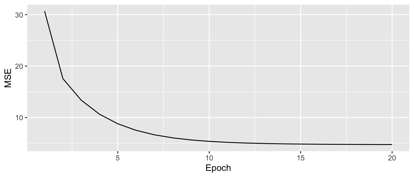

Figure 2.25: Batch Gradient Descent.

We can see that the decrease in the objective function is smoother with Batch Gradient Descend.

2.2.1.3 Mini-Batch Gradient Descent

Even if vectorised implementation can be used to fasten computing with Batch Gradient Descent (which is not possible with Stochastic Gradient Descent), the whole dataset is usually required to be loaded in memory, which can be time consuming.

Another approach, called Mini-Batch Gradient Descent, combines the idea of both Stochastic Gradient Descent and Batch Gradient Descent. In its first step, it consists in creating a batch of observations of smaller size than the entire dataset, called a mini-batch (usually, 64, 128, or 256 observations are used to create a mini batch). Then, the gradient of the objective function is calculated for each observation in the mini batch. The gradients are then averaged and used to update the parameters. A new iteration can then begin with a new mini-batch.

For a given mini-batch, the computations can be vectorised and does not require to have the entire dataset loaded in memory. However, the size of the mini-batches need to be decided on prior the algorithm is launched.

To sum up, the algorithm works as follows:

Mini-Batch Descent Algorithm

Randomly pick n observations from the training sample
For each observation, compute the gradient of the objective function
Compute the mean of the gradients computed in step 2
Update the parameters with the mean gradient from step 3
Repeat from step 1 a given number of times.

At iteration $t$, the parameters are updated as follows:

\[\theta^{(t+1)} = \theta_i^{(t)} - \eta \cdot \frac{1}{n} \sum_{i=1}^{n}\nabla \mathcal{L}\big(\theta^{(t)} ; X_i\big),\] where $n$ is the size of the mini-batch.

Again, let us implement this algorithm with the linear model from earlier.

We need starting values for the parameters:

beta <- c(1,1,1)

Let us use the same learning rate as that was used with the Stochastic Gradient Descent algorithm and the same number of epochs.

learning_rate <- 10^-2
nb_epoch <- 20

We can select a number of observations per batch:

batch_size <- 250

Again, let us keep track of the MSE values after each epoch:

mse_values  <- NULL

Then we can use the following loop:

# pb <- txtProgressBar(min = 1, max=nb_epoch, style=3)
for(i_epoch in 1:nb_epoch){
  # cat("\n----------\nEpoch: ", i_epoch, "\n")
  # Randomly draw a batch
  index <- sample(1:n, size = batch_size, replace=TRUE)
  
  # For each observation in the batch, we need to compute the gradient
  gradients_batch <- rep(0, ncol(X))
  for(i in 1:batch_size){
    gradient_current <- 
      grad(func = obj_function, x=beta, y=y[index[i]], X = X[index[i],])
    gradients_batch <- gradients_batch+gradient_current
  }
  # Then we divide by the number of observations to get the average
  avg_gradients_batch <- gradients_batch/batch_size
  
  # Updating the value
  beta <- beta - learning_rate * avg_gradients_batch
  
  # Just for keeping track (not necessary to run the algorithm)
  # Significantly slows down the algorithm
  cost <- obj_function(beta, y, X)
  mse_values <- c(mse_values, cost)
  # End of keeping track
  
  # setTxtProgressBar(pb, i_epoch)
}

The estimated values:

# True values:
true_beta

## beta_0 beta_1 beta_2 
##    3.0   -2.0    0.5

# Estimated values
(beta_batch <- beta)

## [1]  0.8524989 -1.7747998  0.6444584

As for the Batch Gradient Descent, let us wrap these codes in a function:

#' Performs Batch Gradient Descent for a Linear Model
#' @param par Initial values for the parameters.
#' @param fn A function to be minimized, with first argument the vector
#'           of parameters over which minimisation is to take place.
#'           It should return a scalar result.
#' @param y Target variable.
#' @param X Matrix of predictors.
#' @param learning_rate Learning rate.
#' @param nb_epoch Number of epochs.
#' @param batch_size Batch size.
#' @param silent If TRUE (default), progress information
#'               not printed in the console.
mini_batch_gd <- function(par, fn, y, X, learning_rate=10^-2, nb_epoch=10,
                          batch_size = 128, silent=TRUE){
  mse_values  <- NULL
  n <- nrow(X)
  for(i_epoch in 1:nb_epoch){
    if(!silent) cat("\n----------\nEpoch: ", i_epoch, "\n----------")
    # Randomly draw a batch
    index <- sample(1:n, size = batch_size, replace=TRUE)
    # For each observation in the batch, we need to compute the gradient
    gradients_batch <- rep(0, ncol(X))
    for(i in 1:batch_size){
      gradient_current <- 
        grad(func = fn, x=par, y=y[index[i]], X = X[index[i],])
      gradients_batch <- gradients_batch+gradient_current
    }
    # Then we divide by the number of observations to get the average
    avg_gradients_batch <- gradients_batch/batch_size
    
    # Updating the value
    par <- par - learning_rate * avg_gradients_batch
    
    # Just for keeping track (not necessary to run the algorithm)
    # Significantly slows down the algorithm
    cost <- fn(par, y, X)
    if(!silent) cat("MSE : ", cost, "\n")
    mse_values <- c(mse_values, cost)
    # End of keeping track
  }
  structure(list(par = par, mse_values = mse_values,
                 nb_epoch = nb_epoch,
                 learning_rate = learning_rate,
                 batch_size = batch_size))
}

Let us run the Mini-Batch Gradient Descent algorithm multiple times, varying the number of observations in the mini-batches at each time:

# With 32 obs per mini-batch
start_time_mini_batch_32 <- Sys.time()
mini_batch_32 <- mini_batch_gd(par = c(1,1,1), fn = obj_function, 
                               y = y, X = X, 
                               silent=TRUE, nb_epoch = 20, batch_size = 32)
end_time_mini_batch_32 <- Sys.time()



# With 64 obs per mini-batch
start_time_mini_batch_64 <- Sys.time()
mini_batch_64 <- mini_batch_gd(par = c(1,1,1), fn = obj_function,
                               y = y, X = X, silent=TRUE, 
                               nb_epoch = 20, batch_size = 64)
end_time_mini_batch_64 <- Sys.time()


# With 128 obs per mini-batch
start_time_mini_batch_128 <- Sys.time()
mini_batch_128 <- mini_batch_gd(par = c(1,1,1), fn = obj_function,
                                y = y, X = X, silent=TRUE, 
                                nb_epoch = 20, batch_size = 128)
end_time_mini_batch_128 <- Sys.time()


# With 256 obs per mini-batch
start_time_mini_batch_256 <- Sys.time()
mini_batch_256 <- mini_batch_gd(par = c(1,1,1), fn = obj_function,
                                y = y, X = X, silent=TRUE, 
                                nb_epoch = 20, batch_size = 256)
end_time_mini_batch_256 <- Sys.time()

The estimated parameters:

# True values:
beta

## [1]  0.8524989 -1.7747998  0.6444584

# Estimated values:
mini_batch_32$par

## [1]  0.8851996 -1.7382412  0.7427221

mini_batch_64$par

## [1]  0.8647598 -1.7800043  0.6838670

mini_batch_128$par

## [1]  0.8689784 -1.7547041  0.6840733

mini_batch_256$par

## [1]  0.8557173 -1.7529742  0.6988836

Let us look at the time used to estimate the parameters in each situation. The greater the number of observations, the greater the time taken by the algorithm.

end_time_mini_batch_32-start_time_mini_batch_32

## Time difference of 1.055768 secs

end_time_mini_batch_64-start_time_mini_batch_64

## Time difference of 1.950635 secs

end_time_mini_batch_128-start_time_mini_batch_128

## Time difference of 2.984912 secs

end_time_mini_batch_256-start_time_mini_batch_256

## Time difference of 4.395471 secs

Note: if we pick a mini-batch size of 1, the Mini-Batch Gradient Descent algorithm is the same as the Batch Gradient Descent algorithm.

And let us have a look at the MSE along the epochs:

df_plot <- 
  map_df(list(mini_batch_32, mini_batch_64, mini_batch_128, mini_batch_256), 
         ~tibble(MSE = .$mse_values, 
                 batch_size = .$batch_size, 
                 epoch = 1:(.$nb_epoch)))

ggplot(data = df_plot, mapping = aes(x=epoch, y = MSE)) +
  geom_line(aes(colour = as.factor(batch_size))) +
  labs(x = "Epoch", y = "MSE") +
  scale_colour_discrete("Mini-Batch Size")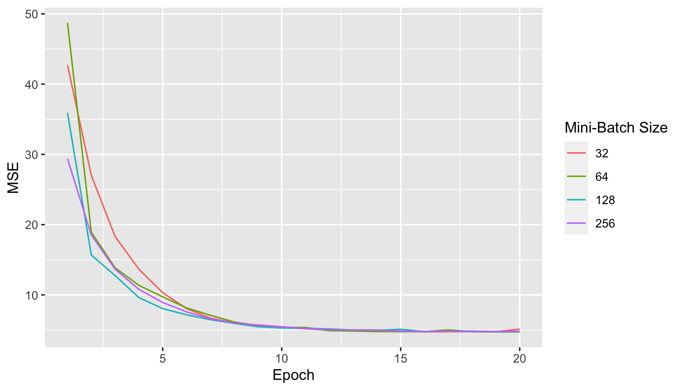

Figure 2.26: Mini-Batch Gradient Descent.

We note that the update process is smoother, less noisier as long as we increase the batch size.

To finish this section, let us have a look at the MSE over the epochs for the different algorithms we used, on the same graph:

df_plot <- 
  tibble(MSE = estim_sgd$mse_values, epoch = 1:estim_sgd$nb_epoch,
         type = "Stochastic Gradient Descent") %>% 
  bind_rows(
    tibble(MSE = estim_batch$mse_values, epoch = 1:estim_batch$nb_epoch,
           type = "Batch Gradient Descent")
  ) %>% 
  bind_rows(
    map_df(list(mini_batch_32, mini_batch_64, 
                mini_batch_128, mini_batch_256), 
           ~tibble(MSE = .$mse_values, 
                   epoch = 1:(.$nb_epoch),
                   type = .$batch_size,)) %>% 
      mutate(type = str_c("Mini-Batch Gradient Descent (size=", type, ")"))
  )

ggplot(data = df_plot, mapping = aes(x=epoch, y = MSE)) +
  geom_line(mapping = aes(colour = type)) +
  labs(x = "Epoch", y = "MSE") +
  scale_colour_manual(values = c(
    "Stochastic Gradient Descent" = "#DDCC77",
    "Batch Gradient Descent" = "#117733",
    "Mini-Batch Gradient Descent (size=32)" = "#44AA99",
    "Mini-Batch Gradient Descent (size=64)" = "#88CCEE",
    "Mini-Batch Gradient Descent (size=128)" = "#DC267F",
    "Mini-Batch Gradient Descent (size=256)" = "#882255"
  )) +
  theme(legend.position = "bottom")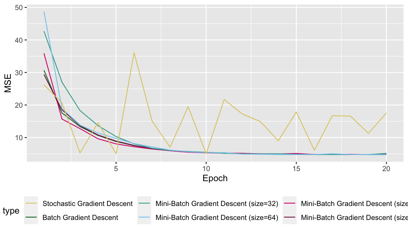

Figure 2.27: Optimisation with different algorithms.

2.2.2 Varying the Learning Rate

So far, we have considered a fixed learning rate $\eta$. The update rule for the $p$ parameters of the objective function we used was the following:

\[\mathbf{\theta}^{(t+1)} = \mathbf{\theta}^{(t)} -\eta \cdot \nabla\mathcal{L}\left(\mathbf{\theta}^{(t)}\right).\] The learning rate may change over the iteration process so that the update rule becomes:

\[\mathbf{\theta}^{(t+1)} = \mathbf{\theta}^{(t)} -\eta_t \cdot \nabla\mathcal{L}\left(\mathbf{\theta}^{(t)}\right),\]

where $\eta_t$ can be set in various ways.

2.2.2.1 Linear Decaying Rate

The learning rate can be set so that it decreases linearly with the number of iterations. In such a case, it is defined as follows:

\[\eta_t = \frac{\eta_t}{t+1}\]

2.2.2.2 Quadratic Decaying Rate

For a quadratically decaying learning rate:

\[\eta_t = \frac{\eta_t}{(t+1)^2}\]

2.2.2.3 Exponential Decaying Rate

For an exponential decay:

\[\eta_t = \eta_t \exp(-\beta t),\] where $\beta>0$.

2.3 Other Algorithms

There are many other algorithms and variants. I would like to sketch two other algorithms in this notebook: Newton’s algorithm and the Coordinate Descent algorithm.

2.3.1 Newton’s Method

When the function to be optimised is convex, doubly differentiable and takes its values in $\mathbb{R}^n$, it is possible to use the second-order derivative to redefine the learning rate.

Taylor’s theorem states that if $\mathcal{L} : \mathbb{R}^p \rightarrow \mathbb{R}$ is twice-differentiable at point $\mathbf{\theta}$, for any small change $\delta\mathbf{\theta}$, the best quadratic approximation to $\mathcal{L}$ is given by the second-order Taylor series:

\[\mathcal{L}(\mathbf{\theta} + \delta\mathbf{\theta}) = \mathcal{L}({\mathbf{\theta}}) + \nabla\mathcal{L}(\mathbf{\theta})^{\top} \delta\mathbf{\theta} + \frac{1}{2} \delta \mathbf{\theta}^\top \mathbf{H} \delta \mathbf{\theta} + \mathcal{O}(\lVert \delta^3\mathbf{\theta} \rVert),\] with $\mathbf{H}=\nabla^2\mathcal{L}(\mathbf{\theta})$ the Hessian matrix

In a similar way as in the case of the best linear approximation, we need to take a step $\delta \mathbf{\theta}$ such that :

\[\mathcal{L}(\mathbf{\theta} + \delta\mathbf{\theta}) < \mathcal{L}(\mathbf{\theta}),\] i.e., for which: \[\delta \mathbf{\theta}^\top \mathbf{H} \delta \mathbf{\theta} < 0\]

With Newton’s method, we will thus take a step along the gradient, and we will use the Hessian matrix to decide the step to take: by doing to, the rate at which we will go down the gradient will account for the convexity of the function.

Newton’s Method

Randomly pick starting values for the parameters
Compute both the gradient and the Hessian of the objective function at the current value of the parameters using all the observations from the training sample
Update the parameters
Repeat from step 2 until a fixed number of iteration or until convergence.

At iteration $t$, the parameters are updated as follows:

\[\mathbf{H}^{(t)} = \nabla^2 \mathcal{L}\big(\theta^{(t)}\big)\]

\[\mathbf{\theta}^{(t+1)} = \mathbf{\theta}^{(t)} - \big(\mathbf{H}^{(t)}\big)^{-1} \cdot \nabla \mathcal{L}\big(\mathbf{\theta}^{(t)}\big),\]

While computing the second-order derivative can be fast if the expression of this function is simple, it can become computationally very expensive otherwise. The computation of the Hessian can also be very challenging when facing a large number of observations ($n^2$ computations are required for the second-order derivative).

Computing the inverse of the Hessian matrix is computationally expensive. The BFGS (Broyden Fletcher Goldfard Shanno) method avoids computing $\mathbf{H}^{-1}$ and instead estimates an approximation of the Hessian matrix.

Let us illustrate the method. Consider the following function:

\[f(x_1, x_2) = (x_1-x_2)^4 + 2x_1^2 + x_2^2 - x_1 + 2x_2\]

x_1 <- seq(-10, 10, by = 0.3)
x_2 <- seq(-10, 10, by = 0.3)
z_f <- function(x_1,x_2) (x_1-x_2)^4 + 2*x_1^2 + x_2^2 - x_1 + 2*x_2
z_f_to_optim <- function(theta){
  x_1 <- theta[1]
  x_2 <- theta[2]
  (x_1-x_2)^4 + 2*x_1^2 + x_2^2 - x_1 + 2*x_2
}
z <- outer(x_1, x_2, z_f)

A graphical representation of this function can be obtained as follows:

par(mar = c(1, 1, 1, 1))
th = 150
pmat <- 
  persp3D(x = x_1, y = x_2, z = z, colkey=F, contour=T,
          ticktype = "detailed", asp = 1, phi = 40, theta = th, 
          border = "grey10", alpha=.4, d = .8,r = 2.8,
          expand = .6, shade = .2,axes = T,box = T,cex = .1)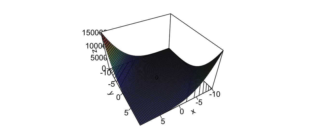

Figure 2.28: Surface of the illustrative function.

Let us pick some starting values:

theta <- c(-9, 9)

The Newton’s Method quickly converges, let us pick a small maximum number of iteration.

nb_max_iter <- 20

Let us set a value for the absolute tolerance:

abstol <- 10^-5

At our starting point, the value of the function is:

(current_obj <- z_f_to_optim(theta))

## [1] 105246

Let us keep a track on our updated values for the vector of parameters:

theta_values <- NULL

Then we can make a loop to update iteratively the vector of parameters.

for(i in 1:nb_max_iter){
  gradient <- grad(func = z_f_to_optim, x = theta)
  H <- hessian(func = z_f_to_optim, x = theta)
  # Updating the parameters
  theta <- theta - t(solve(H) %*% gradient)
  new_obj <- z_f_to_optim(theta)
  # Keeping track
  theta_values <- rbind(theta_values, theta)
  
  if(abs(current_obj - new_obj) < abstol){
    break
  }else{
    current_obj <- new_obj
  }
}

The algorithm stopped after the following number of iterations:

## [1] 13

The algorithm tells us that the minimum is reached at the following point:

theta

##            [,1]       [,2]
## [1,] 0.03349047 -0.5669809

Let us have a look at the updates on a first graph:

par(mar = c(1, 1, 1, 1))
pmat <- 
  persp3D(x = x_1, y = x_2, z = z, colkey=F, contour=T,
          ticktype = "detailed", asp = 1, phi = 40, theta = th,
          border = "grey10", alpha=.4, d = .8,r = 2.8,
          expand = .6, shade = .2,axes = T,box = T,cex = .1)

xx <- theta_values[,1]
yy <- theta_values[,2]
zz <- z_f(xx,yy)
new_point <- trans3d(xx,yy,zz,pmat = pmat)
lines(new_point,pch = 20,col = "red", cex=2)
points(new_point,pch = 20,col = "red", cex=2)
points(map(new_point, last),pch = 20,col = "green", cex=1.5)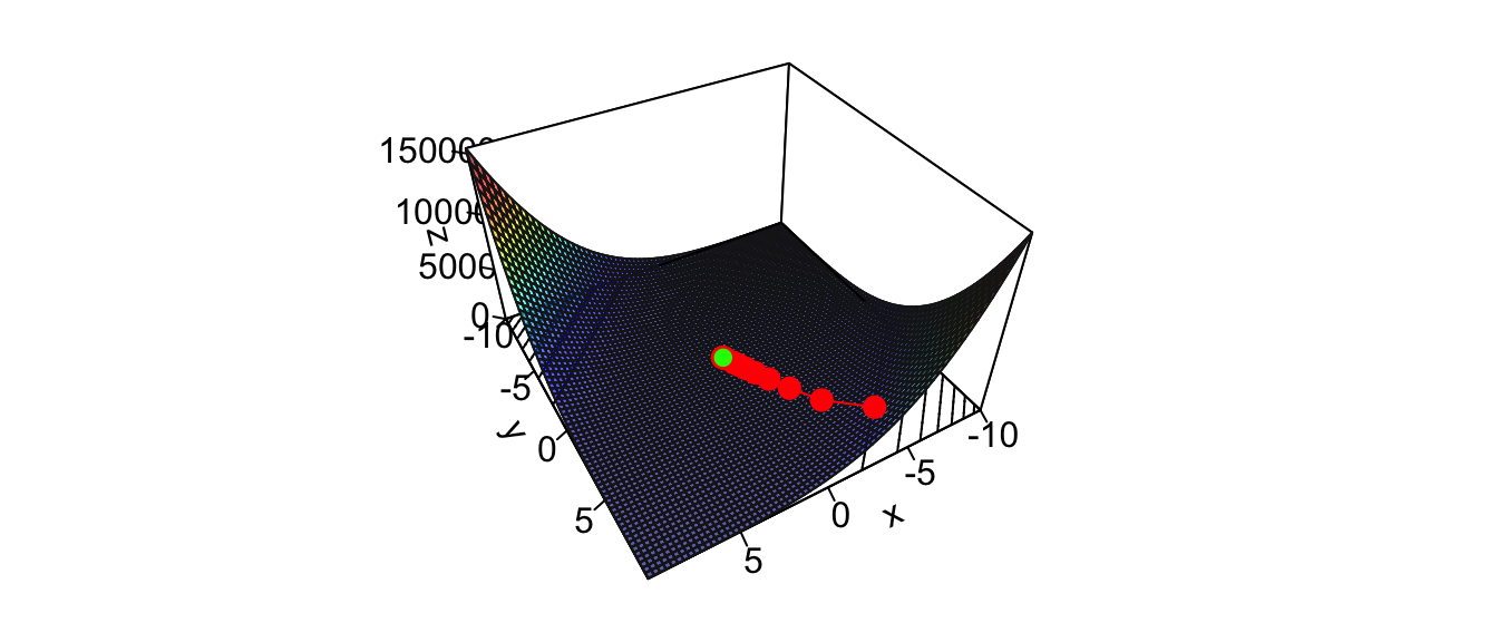

Figure 2.29: Newton’s algorithm: steps of the iterative process.

And on a contour plot:

contour2D(x=x_1, y=x_2, z=z, colkey=F, 
          main="Contour plot", xlab="x_1", ylab="x_2")
for(i in 1:(nrow(theta_values)-1)){
  segments(x0 = theta_values[i, 1], x1 = theta_values[i+1, 1],
           y0 = theta_values[i, 2], y1 = theta_values[i+1, 2], 
           col = "red", lwd=2)
}
points(x=theta_values[,1], y=theta_values[,2], t="p", 
       pch=19, col = "red")
points(x=theta_values[nrow(theta_values),1], 
       y=theta_values[nrow(theta_values),2], t="p", 
       pch=19, col = "green")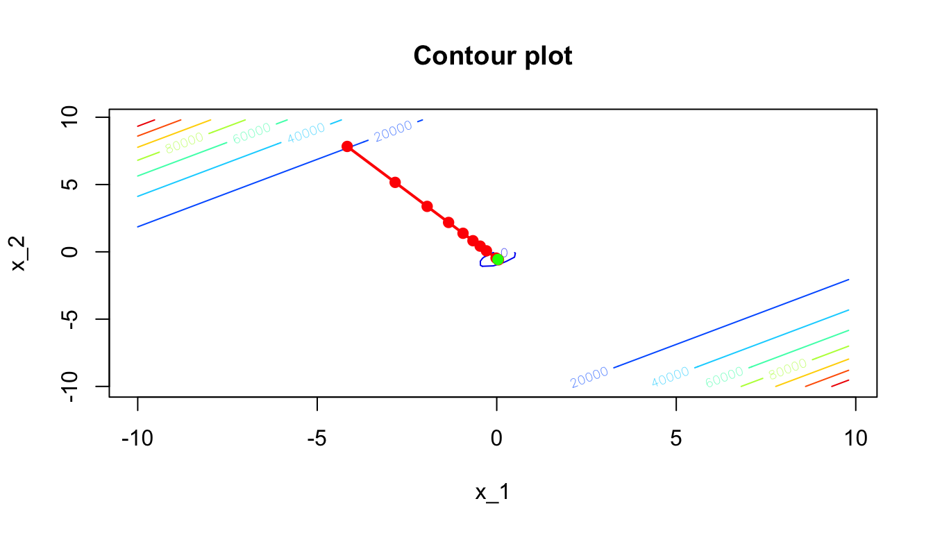

Figure 2.30: Newton’s algorithm: contour plot of the iterative process.

Here, we converged quickly to the minimum, and the computation was really fast. When applying this algorithm to minimise the objective function of a supervised learning task using large datasets, computing the Hessian become way more costly.

To get more details on Newton’s method, see Tibshirani (2019).

2.3.2 Coordinate Descent Algorithm

When trying to optimise a high-dimensional multivariate function, the calculation of each first derivative can quickly become very time consuming.

Intuitively, the $n$-dimensional optimisation problem can be seen as several small $1$-dimensional optimisation problems. The basic idea is to try to minimise over a single dimension at each iteration, keeping all the values of the parameters constant.

More (technical/mathematical) details can be found in the slides titled “Coordinate Descent and Ascent Methods” from Nutini (2015) and in the slides “Optimisation et convexité 1, 2 and 3” from Charpentier (2020) (although the title is in French, the slides are in English, only the videos are in French).

If the function $f$ is convex and differentiable, we can rely on the following theorem to find the minimum:

If $f : \mathbb{R}^n \rightarrow \mathbb{R}$ is convex, differentiable, then :

\[f(\mathbf{x}) \leq f\left( \mathbf{x} + \delta \overrightarrow{\mathbb{e}}_i\right), \forall i \Rightarrow f(\mathbf{x}) = \min\{f\},\]

where $\overrightarrow{\mathbb{e}}_i = (0, \ldots, 0,1,0,\ldots,0)\in \mathbb{R}^n$.

In other words, if we find a point $\mathbf{x}$ such that $f(\mathbf{x})$ is minimised along each of the $n$ coordinate axis, this point is a global minimiser.

We can thus try to find the minimum in each direction instead of looking directly at the problem in $n$ dimensions. We will end up in the global minimum.

The algorithm works the following way:

Coordinate Descent Algorithm

Randomly pick starting values for the parameters
Select a dimension among the $p$ (cyclic sampling, uniform sampling, …)
Compute the first-order derivative of the objective function with respect to the ith parameter
Update the ith parameter
Repeat from step 2 until a fixed number of iteration or until convergence.

Let us first consider a smooth function to illustrate the method: \[f(x_1,x_2) = x_1^2 + x_2^2 + x_1 x_2\]

Let us now generate some observations from that function:

library(plot3D)
library(numDeriv)
n <- 40
x_1 <- x_2 <- seq(-3, 3, length.out=n)
z_f <- function(x_1, x_2) x_1^2 + x_2^2 + x_1*x_2
z_f_to_optim <- function(theta) 
  theta[1]^2 + theta[2]^2 + theta[1]*theta[2]
z <- outer(x_1, x_2, z_f)

We can visualise these observations on a 3D graph:

op <- par()
par(mar = c(1, 1, 1, 1))
flip <- 1
th <- 200
pmat <- 
  persp3D(x = x_1, y = x_2, z = z, colkey=F, contour=T,
          ticktype = "detailed", xlab = "x_1", ylab = "x_2", 
          zlab = "f(x_1, x_2)", asp = 1, phi = 30, theta = th, 
          border = "grey10", alpha=.4, d = .8,r = 2.8,
          expand = .6, shade = .2, axes = T, box = T, cex = .1)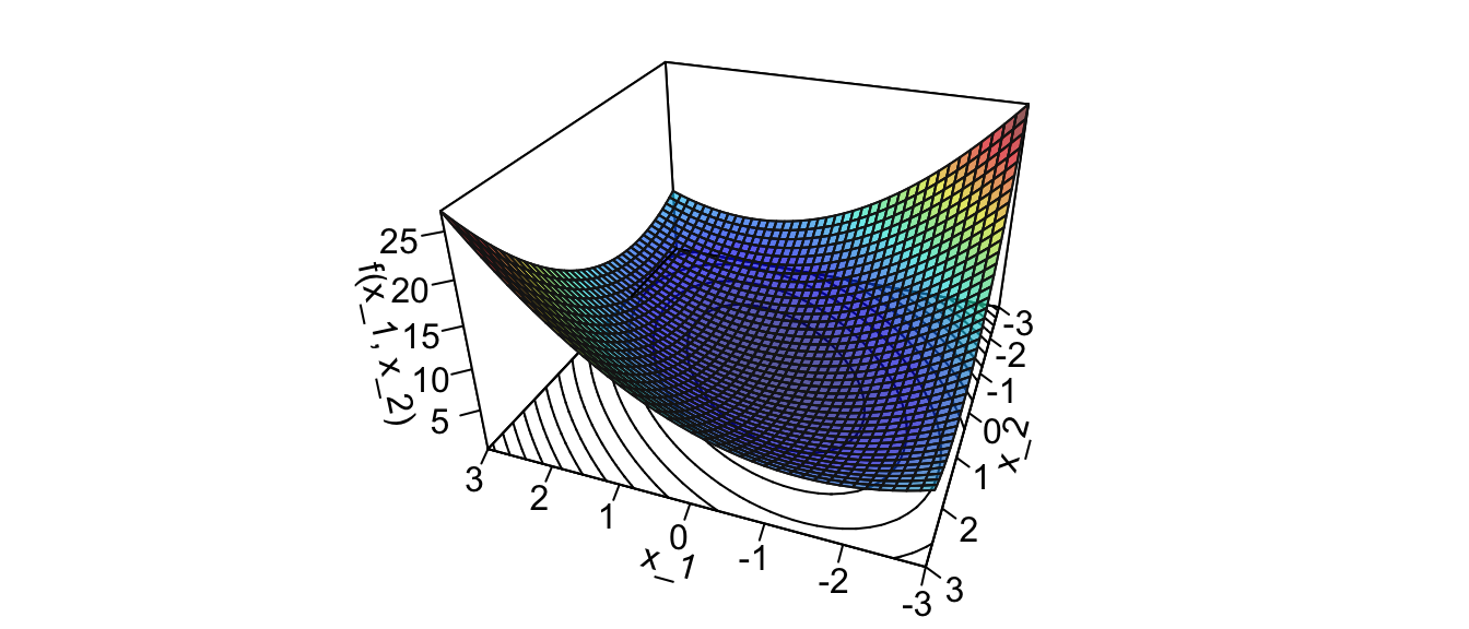

Figure 2.31: Surface of the illustrative spherical function.

Now, let us consider a starting point: $\theta = (2,2.2)$

theta <- c(2, 2.2)

A contour plot can also be used to visualise the process:

contour(x_1, x_1, z, nlevels = 20, xlab = "x_1", ylab = "x_2")
points(theta[1], theta[2], pch = 19, cex = 2, col = "red")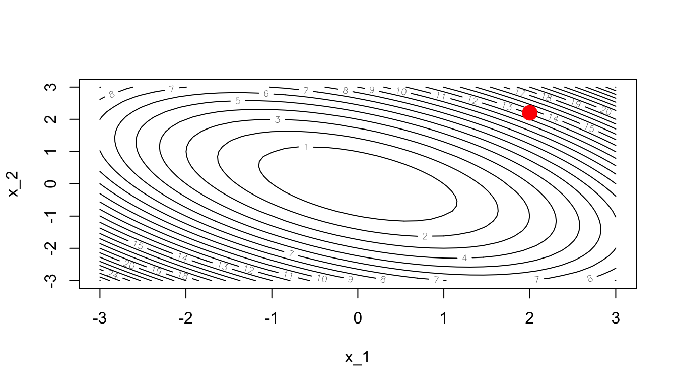

Figure 2.32: Starting point.

We need to minimise over a single dimension. For example, let us begin with the first dimension.

dim_i <- 1

The value of the parameter of the other dimensions (here only the second dimension) will be held fixed. We will only update the first dimension of the parameter.

contour(x_1, x_1, z, nlevels = 20, xlab = "x_1", ylab = "x_2")
abline(h = theta[2], lty=2, col = "blue", lwd=2)
points(theta[1], theta[2], pch = 19, cex = 2, col = "red")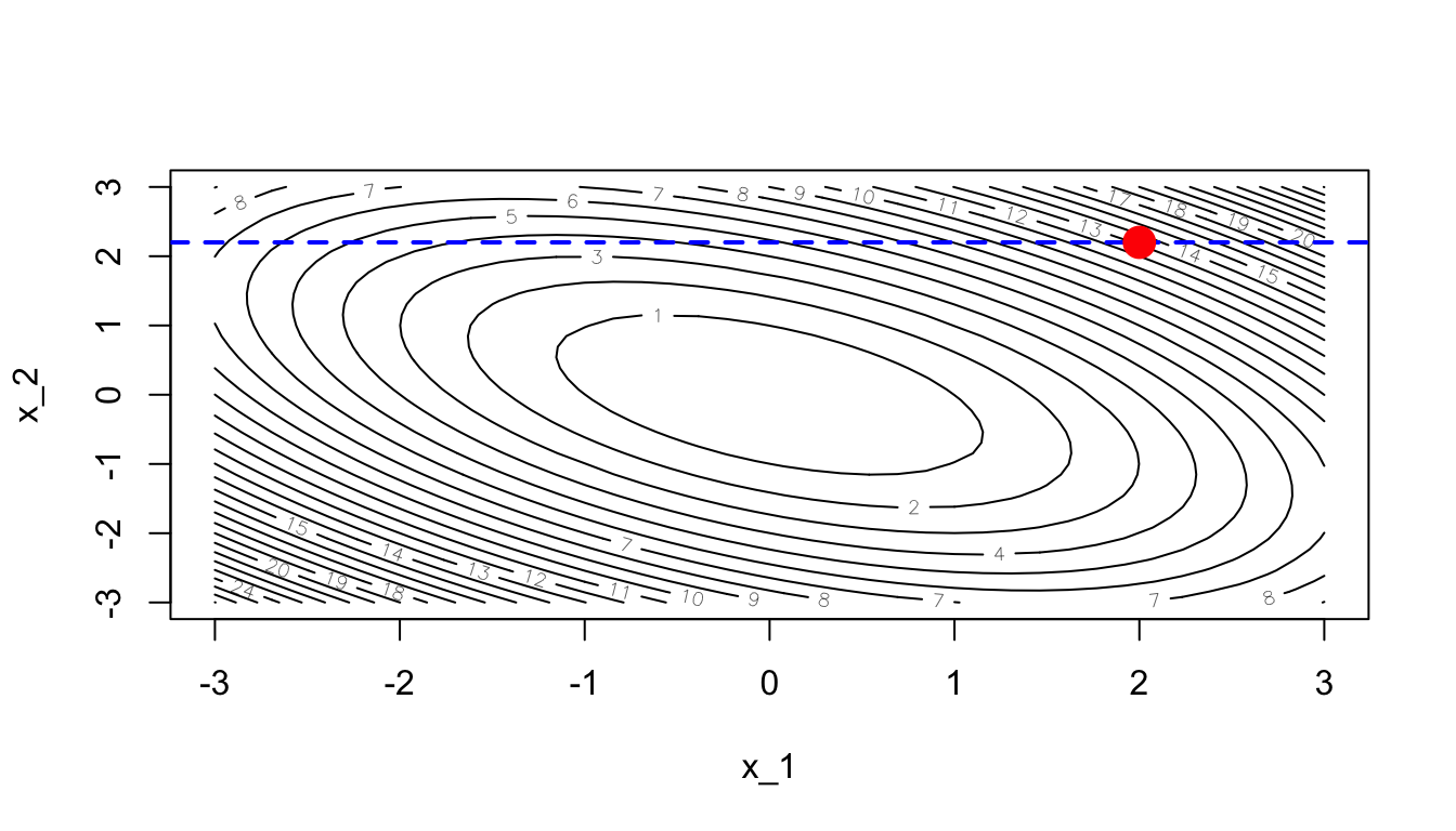

Figure 2.33: Optimisation in a single dimension (dashed blue line).

The first derivative of our function $f$ with respect to $x_1$ writes: \[\frac{\partial f}{\partial x_1}(x_1,x_2) = 2x_1 + x_2.\]

derivative_wrt_x1 <- function(theta){
  2*theta[1] + theta[2]
}

Evaluated at $\theta$:

(grad_i <- derivative_wrt_x1(theta))

## [1] 6.2

Let us select a learning rate:

learning_rate <- 10^-1

The vector of parameters can then be updated:

theta_update <- theta
theta_update[dim_i] <- theta_update[dim_i] - learning_rate * grad_i
theta_update

## [1] 1.38 2.20

Let us keep track of the evolution of the values of $\theta$.

theta_values <- rbind(theta, theta_update)
theta_values

##              [,1] [,2]
## theta        2.00  2.2
## theta_update 1.38  2.2

contour(x_1, x_1, z, nlevels = 20, xlab = "x_1", ylab = "x_2")
abline(h = theta[2], lty=2, col = "blue", lwd = 2)
points(theta[1], theta[2], pch = 19, cex = 2, col = "red")
segments(x0 = theta[1], x1 = theta_update[1],
         y0 = theta[2], y1 = theta_update[2], col = "red", lwd=2)
points(theta_update[1], theta_update[2], pch = 19, cex = 2, col = "red")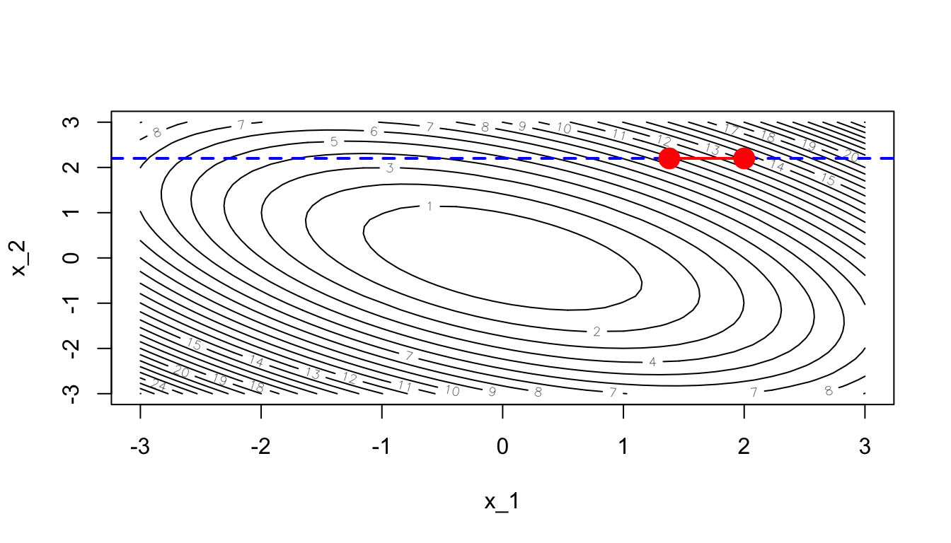

Figure 2.34: Updated value after the first step.

A new iteration can then begin. Let us now consider another dimension:

dim_i <- 2

This time, we will try to optimise on this second dimension only, keeping the values of the other dimension constant.

contour(x_1, x_1, z, nlevels = 20, xlab = "x_1", ylab = "x_2")
abline(v = theta_update[1], lty=2, col = "blue", lwd = 2)
points(theta[1], theta[2], pch = 19, cex = 2, col = "red")
segments(x0 = theta[1], x1 = theta_update[1],
         y0 = theta[2], y1 = theta_update[2], col = "red", lwd=2)
points(theta_update[1], theta_update[2], pch = 19, 
       cex = 2, col = "red")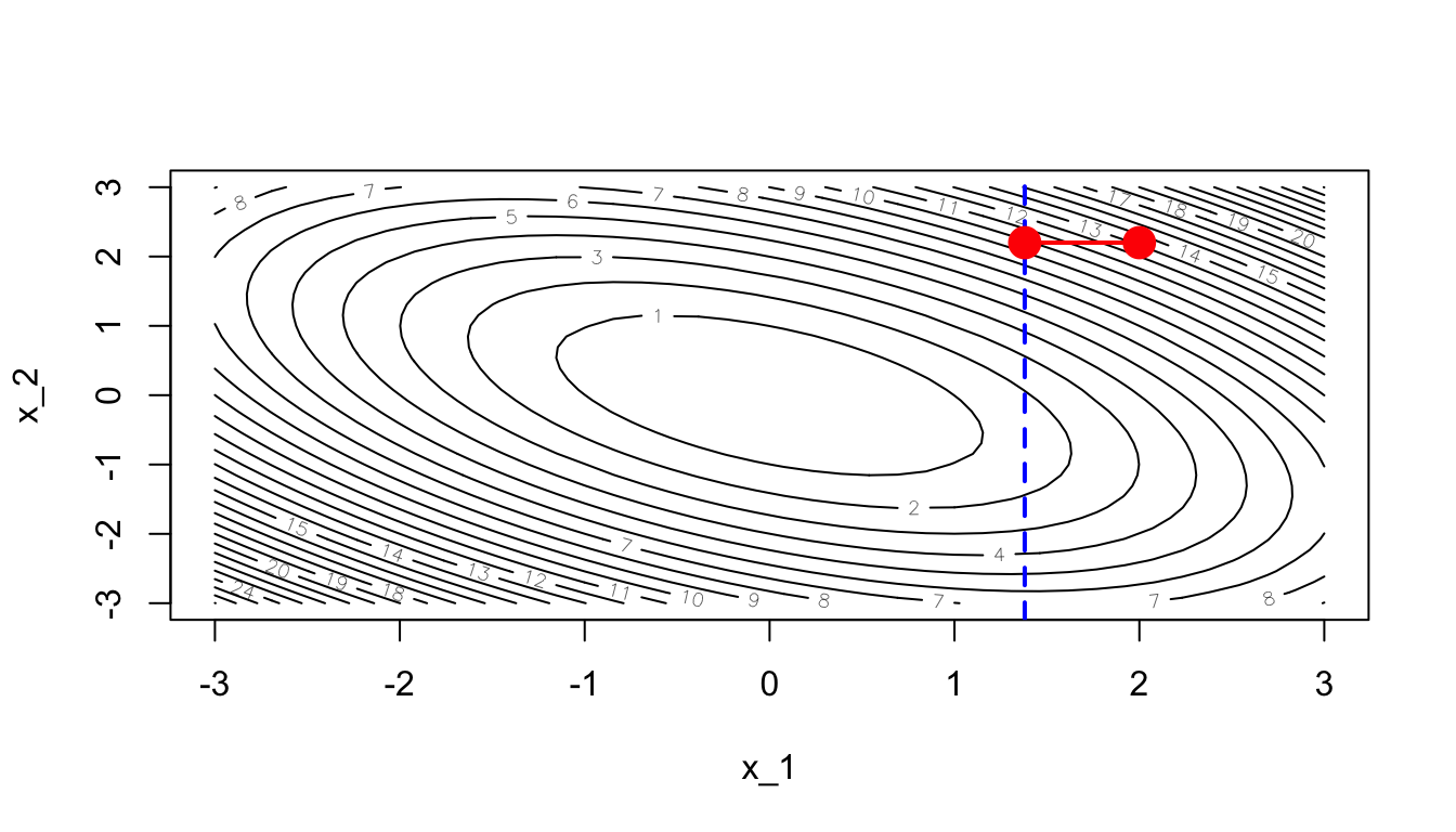

Figure 2.35: Optimisation in another dimension.

The first derivative of our function $f$ with respect to $x_2$ writes: \[\frac{\partial f}{\partial x_2}(x_1,x_2) = 2x_2 + x_1.\]

derivative_wrt_x2 <- function(theta){
  2*theta[2] + theta[1]
}

Evaluated at $\theta$:

(grad_i <- derivative_wrt_x2(theta_update))

## [1] 5.78

The vector of parameters can then be updated:

theta_update[dim_i] <- theta_update[dim_i] - learning_rate * grad_i
theta_update

## [1] 1.380 1.622

Keeping track of the changes:

theta_values <- rbind(theta_values, theta_update)
theta_values

##              [,1]  [,2]
## theta        2.00 2.200
## theta_update 1.38 2.200
## theta_update 1.38 1.622

contour(x_1, x_1, z, nlevels = 20, xlab = "x_1", ylab = "x_2")
abline(v = theta_update[1], lty=2, col = "blue", lwd = 2)
for(i in 1:(nrow(theta_values)-1)){
  segments(x0 = theta_values[i, 1], x1 = theta_values[i+1, 1],
           y0 = theta_values[i, 2], y1 = theta_values[i+1, 2], 
           col = "red", lwd=2)
}
points(theta_values[,1], theta_values[,2], pch = 19, 
       cex = 2, col = "red")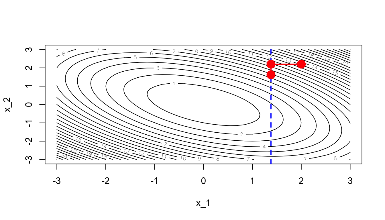

Figure 2.36: Updated value agter the second step.

Then we just need to iterate until a number of iterations is reached or until convergence.

Here is the full code:

# Starting values
theta <- c(2, 2.2)
learning_rate <- 10^-1
abstol <- 10^-5
nb_max_iter <- 100
z_current <- z_f_to_optim(theta)
# To keep track of what happens at each iteration
theta_values <- list(theta)
dims <- NULL

for(i in 1:nb_max_iter){
  
  nb_dim <- length(theta)
  # Cyclic rule to pick the dimension
  dim_i <- (i-1) %% nb_dim + 1
  
  # With uniform sampling
  # dim_i <- sample(x = seq_len(nb_dim), size = 1)
  # Steepest ascent
  if(dim_i == 1){
    grad_i <- derivative_wrt_x1(theta)
  }else{
    grad_i <- derivative_wrt_x2(theta)
  }
  
  # Updating the parameters
  theta_update <- theta
  theta_update[dim_i] <- theta_update[dim_i] - learning_rate * grad_i
  theta <- theta_update
  # To keep track of the changes
  theta_values <- c(theta_values, list(theta))
  dims <- c(dims, dim_i)
  
  # Checking for improvement
  z_updated <- z_f_to_optim(theta_update)
  if(abs(z_updated - z_current) < abstol) break
  z_current <- z_updated
}

The optimisation stopped at iteration:

## [1] 29

theta_values <- do.call("rbind", theta_values)

The final value for the parameter theta is:

theta

## [1] -0.03832741  0.07418966

Let us have a look at the path of the process:

contour(x_1, x_1, z, nlevels = 20, xlab = "x_1", ylab = "x_2")
abline(v = theta_update[1], lty=2, col = "blue", lwd = 2)
for(i in 1:(nrow(theta_values)-1)){
  segments(x0 = theta_values[i, 1], x1 = theta_values[i+1, 1],
           y0 = theta_values[i, 2], y1 = theta_values[i+1, 2], 
           col = "red", lwd=2)
}
points(theta_values[,1], theta_values[,2], pch = 19, 
       cex = .8, col = "red")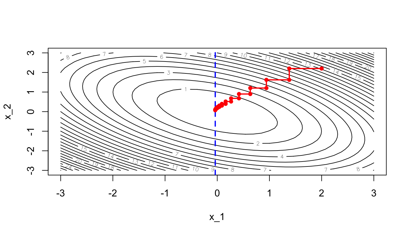

Figure 2.37: Coordinate descent algorithm: iterative process.

Or with the 3D graph:

saveGIF({
  
  for(j in c(rep(1,5), 2:(nrow(theta_values)-1), rep(nrow(theta_values), 10))){
    
    par(mar = c(1, 1, 1, 1))
    flip <- 1
    th <- 200
    pmat <- 
      persp3D(x = x_1, y = x_2, z = z, colkey=F, contour=T, 
              ticktype = "detailed", asp = 1, phi = 30, theta = th, 
              border = "grey10", alpha=.4, d = .8,r = 2.8,
              expand = .6, shade = .2, axes = T, box = T, cex = .1,
              main = paste0("Step ", j))
    
    xx <- theta_values[1:j,1]
    yy <- theta_values[1:j,2]
    zz <- z_f(xx,yy)
    new_point <- trans3d(xx,yy,zz,pmat = pmat)
    lines(new_point,pch = 20,col = "red", cex=2, lwd=2)
    points(new_point,pch = 20,col = "red", cex=2)
  }
  
}, movie.name = "coordinate_descent_contour_3D.gif", interval = 0.01,
ani.width = 720, ani.height = 480)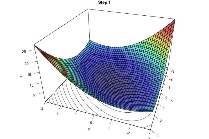

Figure 2.38: Animated version of the iterations of the coordinate descent algorithm.

In this example, we have considered a cyclic sampling rule to decide the dimension to optimise over. Different rules exist. For example, one could use a uniform sampling rule.

2.3.2.1 When the Function to Optimize is not Differentiable in all Points

The coordinate descent algorithm will not be able to find the minimum of a non-differentiable function. The theorem we used in the case where $f$ is convex AND differentiable cannot be used anymore.

It is however possible to find the minimum of some non-differentiable functions using a slightly modified version of the coordinate descent algorithm, if some conditions on the $f$ function are met.

More precisely, if the function $f : \mathbb{R}^n \rightarrow \mathbb{R}$ is not differentiable at all points but can be written as follows: \[f(\mathbf{x}) = g(\mathbf{x}) + \sum_{i=1}^n h_i(\mathbf{x}_i),\] where $g$ is convex and differentiable and where $h_i$ is convex and non-differentiable, then: \[f(\mathbf{x}) \leq f\left(\mathbf{x} + \delta \overrightarrow{\mathbf{e}}_i\right), \forall i \Rightarrow f(\mathbf{x}) = \min\{f\},\] where $\overrightarrow{\mathbf{e}}_i =(0, \ldots,0,1,0, \ldots, 0) \in \mathbb{R}^n$.

Let us consider the following function:

\[f(x_1, x_2) = \underbrace{x_1^2 + x_2^2}_{\text{convex and differentiable}} + \underbrace{\mid x_1 \mid + \mid x_2 \mid}_{\text{convex and non-differentiable}}\]

Let us visualise a graphical representation of this function:

n <- 25
x_1 <- x_2 <- seq(-3, 3, length.out=n)
z_f <- function(x_1, x_2) x_1^2+x_2^2 + abs(x_1) + abs(x_2)
z_f_to_optim <- function(theta) 
  theta[1]^2+theta[2]^2 + abs(theta[1])+abs(theta[2])
z <- outer(x_1, x_2, z_f)

To compute the numerical partial first-order derivative with respect to the ith variable, we can create a function that will numerically estimate the value. Recall that the partial first-order derivative of function $f$ is defined as: \[\frac{\partial f}{\partial x_i}(\mathbf{x}) = \lim_{h\to 0} \frac{f(\mathbf{x}+h\mathbf{e}_i) - f(\mathbf{x})}{h},\]

where $\mathbf{x} = (x_1, \ldots, x_{i-1}, x_i, x_{i+1}, \ldots, x_n) \in \mathbb{R}^n$ and $\mathbf{e}_i = (0, \ldots,0,1,0, \ldots, 0) \in \mathbb{R}^n$.

In R, we can define the following function to numerically estimate the first-order partial derivative:

#' Numerical partial first-order derivative of a function
#' @param par Initial values for the parameters
#' @param fn A function to be derived. It should return a scalar result.
#' @param dim Direction for the derivative (1 to compute the first derivative
#' with respect to the first parameter, 2 to compute the first derivative
#' with respect to the second parameter, etc.)
#' @param nb_dim number of dimensions
num_first_deriv <- function(par, fn, dim, nb_dim){
  h <- par[dim]*sqrt(10^-12)
  e <- rep(0, nb_dim) ; e[dim_i] <- 1
  (fn(par+h*e) - fn(par))/h
}

Then, we can run the coordinate descent algorithm:

# Starting values
theta <- c(2, 2.2)
learning_rate <- 10^-1
abstol <- 10^-6
nb_max_iter <- 500
z_current <- z_f_to_optim(theta)
# To keep track of what happens at each iteration
theta_values <- list(theta)
dims <- NULL


for(i in 1:nb_max_iter){
  
  nb_dim <- length(theta)
  # Cyclic rule to pick the dimension
  dim_i <- (i-1) %% nb_dim + 1
  
  # Partial derivative wrt to the dim_i axis
  grad_i <- 
    num_first_deriv(par = theta, fn = z_f_to_optim, 
                    dim = dim_i, nb_dim = nb_dim)
  
  # Updating the parameters
  theta_update <- theta
  theta_update[dim_i] <- theta_update[dim_i] - learning_rate * grad_i
  theta <- theta_update
  # To keep track of the changes
  theta_values <- c(theta_values, list(theta))
  dims <- c(dims, dim_i)
  
  # Checking for improvement
  z_updated <- z_f_to_optim(theta_update)
  if(abs(z_updated - z_current) < abstol) break
  z_current <- z_updated
}

theta

## [1] 0.05555447 0.05555593

theta_values <- do.call("rbind", theta_values)

Looking at the path followed by the updated parameters during the iterations:

contour(x_1, x_1, z, nlevels = 20, xlab = "x_1", ylab = "x_2")
for(i in 1:(nrow(theta_values)-1)){
  segments(x0 = theta_values[i, 1], x1 = theta_values[i+1, 1],
           y0 = theta_values[i, 2], y1 = theta_values[i+1, 2], 
           col = "red", lwd=2)
}
points(theta_values[,1], theta_values[,2], pch = 19,
       cex = .8, col = "red")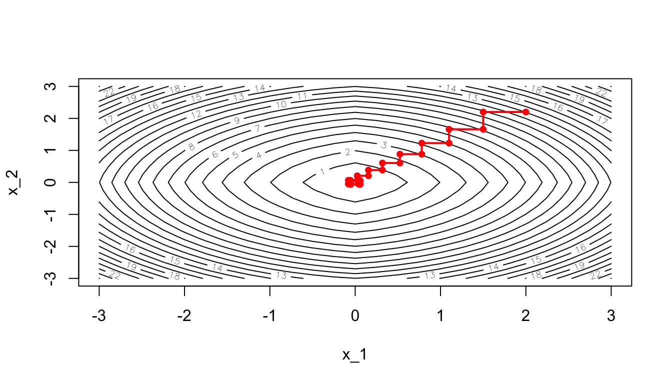

Figure 2.39: Coordinate descent: iterative process if the function is not differentiable in all points.

References

Charpentier, Arthur. 2020. “Act6100 Analyse Des Données En Actuariat.” https://github.com/freakonometrics/ACT6100.

Nutini, Julie. 2015. “Coordinate Descent and Ascent Methods.” https://www.cs.ubc.ca/labs/lci/mlrg/slides/mlrg_CD.pdf.

Tibshirani, Ryan. 2019. “Convex Optimization Course.” https://www.stat.cmu.edu/~ryantibs/convexopt/.