3 Overfitting
This notebook illustrates the notion of overfitting through three examples. In the first example, the idea is to build a a classifier on some real data and to assess the predictive capabilities of the model on seen data, and then on unseen data. In the second example and third, the idea is to see how overfitting may lead us to select a hyperparameter of a machine learning model that may exhibit the best results on seen data but will produce a model that performs less well on unseen data.
Through these examples, the notion of cross validation will be recalled.
3.1 First Example: Default of Credit Card
Disclaimer: The idea of this session is taken from Demšar (2021).
In this first example, we will use a logistic regression to predict the default of credit card clients. The data used here come from Yeh and Lien (2009). They can be downloaded for free on the UCI Machine Learning Repository.
On the repository, the following information about the dataset is provided:
This research aimed at the case of customers’ default payments in Taiwan and compares the predictive accuracy of probability of default among six data mining methods. From the perspective of risk management, the result of predictive accuracy of the estimated probability of default will be more valuable than the binary result of classification - credible or not credible clients. Because the real probability of default is unknown, this study presented the novel “Sorting Smoothing Method” to estimate the real probability of default. With the real probability of default as the response variable (Y), and the predictive probability of default as the independent variable (X), the simple linear regression result (Y = A + BX) shows that the forecasting model produced by artificial neural network has the highest coefficient of determination; its regression intercept (A) is close to zero, and regression coefficient (B) to one. Therefore, among the six data mining techniques, artificial neural network is the only one that can accurately estimate the real probability of default.
The target variable (y) is the default payment the next month (Yes = 1, No = 0). There are 23 features at hand.
LIMIT_BAL: Amount of the given credit (NT dollar): it includes both the individual consumer credit and his/her family (supplementary) credit.SEX: Binary Coded Gender (1 = male, 2 = female)EDUCATION: Education (1 = graduate school; 2 = university; 3 = high school; 4 = others)MARRIAGE: Marital status (1 = married; 2 = single; 3 = others)AGE: Age (year)PAY_0,PAY_1, …,PAY_6: History of past payment.- -1 = pay duly;
- 1 = payment delay for one month;
- 2 = payment delay for two months; …
- 8 = payment delay for eight months;
- 9 = payment delay for nine months and above.
Past monthly payment records (from April to September, 2005) tracked as follows:
PAY_0: repayment in September, 2005PAY_1: repayment in August, 2005- …
PAY_6: repayment in April, 2005
BILL_AMT1, …,BILL_AMT6: Amount of bill statement (NT dollar).BILL_AMT1: in September, 2005BILL_AMT2: in August, 2005- …
BILL_AMT6: in April, 2005
PAY_AMT1, …,PAY_AMT6: Amount of previous payment (NT dollar).PAY_AMT1: amount paid in September, 2005PAY_AMT2: amount paid in August, 2005- …
PAY_AMT6: amount paid in April, 2005
Let us load the data:
library(tidyverse)
library(readxl)
paste0(
  "https://egallic.fr/Enseignement/ML/ECB/",
  "data/default_credit_card_clients.xls") %>%
  download.file(destfile = "default_credit_card_clients.xls")

df <- read_excel("default_credit_card_clients.xls", skip = 1)
Let us rename the target variable:
df <-
  df %>%
  rename(y = `default payment next month`)
df
## # A tibble: 30,000 × 25
## ID LIMIT_BAL SEX EDUCATION MARRIAGE AGE PAY_0 PAY_2 PAY_3 PAY_4 PAY_5
## <dbl> <dbl> <dbl> <dbl> <dbl> <dbl> <dbl> <dbl> <dbl> <dbl> <dbl>
## 1 1 20000 2 2 1 24 2 2 -1 -1 -2
## 2 2 120000 2 2 2 26 -1 2 0 0 0
## 3 3 90000 2 2 2 34 0 0 0 0 0
## 4 4 50000 2 2 1 37 0 0 0 0 0
## 5 5 50000 1 2 1 57 -1 0 -1 0 0
## 6 6 50000 1 1 2 37 0 0 0 0 0
## 7 7 500000 1 1 2 29 0 0 0 0 0
## 8 8 100000 2 2 2 23 0 -1 -1 0 0
## 9 9 140000 2 3 1 28 0 0 2 0 0
## 10 10 20000 1 3 2 35 -2 -2 -2 -2 -1
## # … with 29,990 more rows, and 14 more variables: PAY_6 <dbl>, BILL_AMT1 <dbl>,
## # BILL_AMT2 <dbl>, BILL_AMT3 <dbl>, BILL_AMT4 <dbl>, BILL_AMT5 <dbl>,
## # BILL_AMT6 <dbl>, PAY_AMT1 <dbl>, PAY_AMT2 <dbl>, PAY_AMT3 <dbl>,
## # PAY_AMT4 <dbl>, PAY_AMT5 <dbl>, PAY_AMT6 <dbl>, y <dbl>3.1.1 Somme Summary Statistics on the Whole Dataset
Let us have a really quick glance at the dataset. For a more accurate estimate, data cleaning and feature engineering would be necessary. As this is not the point of this notebook, we will pretend not to have seen the issues that will be visible in the descriptive statistics.
Feel free to skip this part to get to the main point of the notebook.
The dimensions of the table are the following:
dim(df)## [1] 30000 25We note that the dataset is not balanced:
df %>%
  group_by(y) %>%
  count() %>%
  arrange(desc(n))
## # A tibble: 2 × 2
## # Groups: y [2]
## y n
## <dbl> <int>
## 1 0 23364
## 2 1 6636Let us visualise this on a barplot:
df %>%
  mutate(y=factor(y, levels = c(1,0), labels = c("Yes", "No"))) %>%
  ggplot(data = .) +
  geom_bar(stat = "count", aes(y = y)) +
  labs(x = "Frequency", y = NULL) +
  theme(plot.title.position = "plot")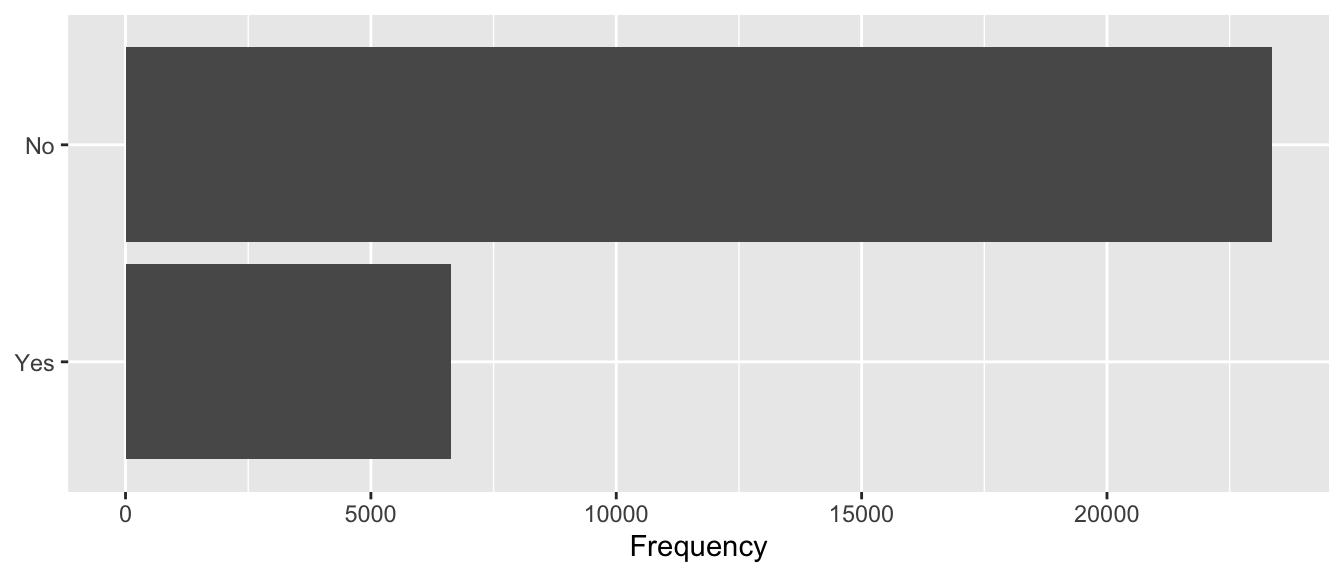
Figure 3.1: Default payment the next month.
We do not have thousands of predictors here, so we can have a little fun with the descriptive statistics. Let us create a table that associates a label to each variable and provides its type (numeric, qualitative or ordinal).
c(
  "y", "Default payment the next month", "qualitative",
  "ID", "ID number", "numeric",
  "LIMIT_BAL", "Amount of the given credit", "numeric",
  "SEX", "Gender", "qualitative",
  "EDUCATION", "Education", "ordinal",
  "MARRIAGE", "Marital status", "qualitative",
  "AGE", "Age", "numeric",
  "PAY_0", "Repayment status September", "qualitative",
  "PAY_2", "Repayment status August", "qualitative",
  "PAY_3", "Repayment status July", "qualitative",
  "PAY_4", "Repayment status June", "qualitative",
  "PAY_5", "Repayment status May", "qualitative",
  "PAY_6", "Repayment status April", "qualitative",
  "BILL_AMT1", "Bill amount September", "numeric",
  "BILL_AMT2", "Bill amount August", "numeric",
  "BILL_AMT3", "Bill amount July", "numeric",
  "BILL_AMT4", "Bill amount June", "numeric",
  "BILL_AMT5", "Bill amount May", "numeric",
  "BILL_AMT6", "Bill amount April", "numeric",
  "PAY_AMT1", "Amount previous payment September", "numeric",
  "PAY_AMT2", "Amount previous payment August", "numeric",
  "PAY_AMT3", "Amount previous payment July", "numeric",
  "PAY_AMT4", "Amount previous payment June", "numeric",
  "PAY_AMT5", "Amount previous payment May", "numeric",
  "PAY_AMT6", "Amount previous payment April", "numeric") %>%
  matrix(ncol = 3, byrow = TRUE) %>%
  as_tibble() %>%
  magrittr::set_colnames(c("variable", "label", "type")) ->
  variable_names_df
We can look at the values of our predictors depending on the response variable. Let us perform some basic parametric tests to see whether the distribution of each feature differs depending on the response variable.
#' format_p_value
#' Format the p-value so that it displays "<10^{i}", if i <= 3
#' rounds the value with 2 digits otherwise
#' @param x p-value to format
#' x <- 0.000133613 ; x <- 0.0011
format_p_value <- function(x){

  if(x < 10^-3){
    resul <- str_c("**< 10^{-3}**")
  }else if(x > 10^-3){
    if(x < 0.05){
      resul <- str_c("**", round(x, 3), "**")
    }else{
      resul <- round(x, 3)
    }
  }else{
    resul <- "**0.001**"
  }

  resul
}
We can create a rather big function to create a table with summary statistics, depending on the type of each variable and on the response variable.
#' Compute descriptive statistics on `df` grouped by `grouping_var`
#' depending on the type of the variable of interest
#' (qualitative, ordinal, numerical)
#' Then performs test of equality of mean/proportion on the sub-samples.
#'
#' @param variable (string) name of the variable of interest
#' @param grouping_var (string) name of the qualitative variable
#'                     that defines groups
#' @param variable_names table with three columns:
#'                       1- variable name, 2- label, 3-type
sample_diff <- function(variable, df,
                        grouping_var,
                        variable_names = variable_names_tlm){

  label_variable <-
    variable_names %>% filter(variable == !!variable) %>%
    magrittr::extract2("label")
  type <-
    variable_names %>% filter(variable == !!variable) %>%
    magrittr::extract2("type")

  if(type %in% c("qualitative", "ordinal")){

    whole_sample <-
      df %>%
      filter(!is.na(!!!syms(variable)), !is.na(!!!syms(grouping_var))) %>%
      mutate(label = label_variable) %>%
      select(label, !!!variable) %>%
      group_by(label, !!!syms(variable)) %>%
      summarise(n = n(), .groups = "drop")

    nb_tot <- sum(whole_sample$n)

    whole_sample <-
      whole_sample %>%
      mutate(pct = n / sum(n),
             pct = (round(100*pct, 2)) %>% str_c("(", ., "%)")) %>%
      unite(`Whole Sample`, n, pct, sep = " ")

    subsamples <-
      df %>%
      filter(!is.na(!!!syms(variable)), !is.na(!!!syms(grouping_var))) %>%
      mutate(label = label_variable) %>%
      select(label, !!!variable, !!!grouping_var) %>%
      group_by(label, !!!syms(variable), !!!(syms(grouping_var))) %>%
      summarise(n = n(), .groups = "drop") %>%
      group_by(!!!syms(grouping_var)) %>%
      mutate(pct = n / sum(n),
             pct = (round(100*pct, 2)) %>% str_c("(", ., "%)")) %>%
      unite(value, n, pct, sep = " ")

    res <-
      whole_sample %>%
      left_join(subsamples) %>%
      ungroup() %>%
      spread_(key_col = grouping_var,  value_col = "value",
              fill = "0 (0.00%)") %>%
      mutate(label = ifelse(
        row_number() == 1,
        yes = str_c(label,
                    " (n = ", format(nb_tot, big.mark = ","), ")"),
        no = label)) %>%
      unite(label, label, !!!variable, sep = " ")

  }else{

    whole_sample <-
      df %>%
      filter(!is.na(!!!syms(variable)), !is.na(!!!syms(grouping_var))) %>%
      mutate(label = label_variable) %>%
      select(label, !!!variable)

    nb_tot <- nrow(whole_sample)

    whole_sample <-
      whole_sample %>%
      group_by(label) %>%
      summarise(mean = mean(!!!syms(variable), na.rm = TRUE) %>%
                  formatC(format = "e", digits = 2),
                sd = sd(!!!syms(variable), na.rm = TRUE) %>%
                  formatC(format = "e", digits = 2),
                .groups = "drop") %>%
      mutate(sd = str_c("(+/-", sd, ")")) %>%
      unite(`Whole Sample`, mean, sd, sep = " ")


    subsamples <-
      df %>%
      filter(!is.na(!!!syms(variable)), !is.na(!!!syms(grouping_var))) %>%
      mutate(label = label_variable) %>%
      select(label, !!!variable, !!!grouping_var) %>%
      group_by(label, !!!syms(grouping_var)) %>%
      summarise(mean = mean(!!!syms(variable)) %>%
                  formatC(format = "e", digits = 2),
                sd = sd(!!!syms(variable)) %>%
                  formatC(format = "e", digits = 2),
                .groups = "drop") %>%
      mutate(sd = str_c("(+/-", sd, ")")) %>%
      unite(value, mean, sd, sep = " ")

    res <-
      whole_sample %>%
      left_join(subsamples) %>%
      ungroup() %>%
      spread_(key_col = grouping_var,  value_col = "value", fill = "0 (+/-0.00)") %>%
      mutate(label = ifelse(
        row_number() == 1,
        yes = str_c(label,
                    " (n = ", format(nb_tot, big.mark = ","), ")"),
        no = label))
  }

  if(type == "qualitative"){
    chisq_test <- chisq.test(df %>% magrittr::extract2(grouping_var),
                             df %>% magrittr::extract2(variable))
    p_value <- chisq_test$p.value
  }else if(type == "ordinal"){
    kruskal_test <- kruskal.test(str_c(grouping_var, "~", variable) %>%
                                   as.formula(), data = df)
    p_value <- kruskal_test$p.value
  }else{
    # Numerical
    form <- str_c(variable, " ~ ", grouping_var) %>% as.formula()
    anov <- aov(form, data = df)
    anov_summary <-  anov %>% summary() %>% .[[1]]
    p_value <- anov_summary$`Pr(>F)`[1]
  }

  # Adding stars for p-values
  p_value <- format_p_value(p_value)

  resul <- res %>%
    mutate(`p value` = c(rep("", nrow(res)-1), p_value))
  resul
}# End of sample_diff()
Let us apply this function to all our predictors:
df_summary_stats <-
  variable_names_df$variable[!variable_names_df$variable%in%c("y", "ID")]%>%
  map_df(sample_diff, df = df,
         grouping_var = "y", variable_names = variable_names_df)
Now we can print the summary table:
library(kableExtra)
df_summary_stats %>%
  kableExtra::kable(caption = "Driving habits before and after the claim",
                    format = "latex", longtable = TRUE) %>%
  kableExtra::kable_classic(full_width = F, html_font = "Cambria") %>%
  kableExtra::kable_styling(
    bootstrap_options = c("striped", "hover", "condensed", "responsive"),
    font_size = 6)
3.1.2 Fitting the Model
Let us take a sample of the data such that the number of predictors is about the same order of magnitude as the number of rows. We will create a dataset with only 50 observations here.
set.seed(134)
# Number of observations
n <- 50
df_first_example <-
  sample_n(df %>% filter(y == 0), size = n/2, replace= FALSE) %>%
  bind_rows(
    sample_n(df %>% filter(y == 1), size = n/2, replace= FALSE)
  ) %>%
  select(-ID)
We will use a logistic regression to try to predict the credit card default clients. Please note that we do it very naively here, without considering, for example, that some data are categorical.
Let us use all the 23 predictors in the model.
reg <- glm(y ~ ., data = df_first_example, family = "binomial")For convenience, we can define two functions:
confusion_table: a function that constructs the confusion tablecompute_metric_confusion: a function that computes errors metrics from the confusion matrix
#' Get the confusion table
#' @param observed vector of observed values
#' @param predicted vector of predicted values
confusion_table <- function(observed, predicted){
  confusion_matrix <- table(observed, predicted)
  confusion_matrix_prop <- prop.table(confusion_matrix)
  confusion_matrix_print <- confusion_matrix
  for(i in 1:ncol(confusion_matrix_print)){
    for(j in 1:nrow(confusion_matrix_print)){
      confusion_matrix_print[i,j] <-
        str_c(confusion_matrix_print[i,j], " (",
              confusion_matrix_prop[i,j], "%)")
    }
  }
  metrics <- compute_metric_confusion(confusion_matrix)
  list(confusion_matrix = confusion_matrix,
       confusion_matrix_print = confusion_matrix_print,
       metrics = metrics)
}
#' Computes errors metrics from the confusion matrix
#' @param confusion_matrix Confusion matrix
compute_metric_confusion <- function(confusion_matrix){
true_negative <- confusion_matrix["0", "0"]
if(is.null(true_negative)) true_negative <- 0
false_positive <- confusion_matrix["0", "1"]
if(is.null(false_positive)) false_positive <- 0
false_negative <- confusion_matrix["1", "0"]
if(is.null(false_negative)) false_negative <- 0
true_positive <- confusion_matrix["1", "1"]
if(is.null(true_positive)) true_positive <- 0
error_rate <- (false_positive+false_negative)/sum(confusion_matrix)
# True positive rate
TPR <- true_positive / (true_positive + false_negative)
# False positive rate
FPR <- false_positive / (false_positive + true_negative)
# True negative rate
TNR <- true_negative / (true_negative + false_positive)
# False negative rate
FNR <- false_negative / (false_negative + true_positive)
# Overall error rate
OER <- (false_negative + false_positive) /
(false_negative + false_positive + true_positive + true_negative)
list(`Erorr rate` = error_rate,
`True positive rate` = TPR,
`False positive rate` = FPR,
`True negative rate` = TNR,
`False negative rate` = FNR,
`Overall error rate` = OER
)
}Now, let us have a look at the predictive capabilities of our model:
# Predictions:
threshold <- .5
pred_prob <- predict(reg)
pred <- ifelse(pred_prob>.5, 1, 0)
We can easily obtain the confusion matrix and some error metrics with our function:
confusion_matrix <- confusion_table(df_first_example$y, pred)Here is the confusion matrix:
confusion_matrix$confusion_matrix_print## predicted
## observed 0 1
## 0 23 (0.46%) 2 (0.04%)
## 1 6 (0.12%) 19 (0.38%)And the metrics:
confusion_matrix$metrics## $`Erorr rate`
## [1] 0.16
##
## $`True positive rate`
## [1] 0.76
##
## $`False positive rate`
## [1] 0.08
##
## $`True negative rate`
## [1] 0.92
##
## $`False negative rate`
## [1] 0.24
##
## $`Overall error rate`
## [1] 0.16With 50 observations and 23 regressors, we do not make that many mistakes.
3.1.3 Randomly Assigning the Classes
Now, let us try something. We will keep the observations unchanged, excepts for the value of the target value. The latter will be randomly drawn. We will store the new target variable in a column named y_new in the data table.
set.seed(123)
df_first_example <-
  df_first_example %>%
mutate(y_new = sample(c(0, 1), size = n(), replace = TRUE))df_first_example$y## [1] 0 0 0 0 0 0 0 0 0 0 0 0 0 0 0 0 0 0 0 0 0 0 0 0 0 1 1 1 1 1 1 1 1 1 1 1 1 1
## [39] 1 1 1 1 1 1 1 1 1 1 1 1df_first_example$y_new## [1] 0 0 0 1 0 1 1 1 0 0 1 1 1 0 1 0 1 0 0 0 0 1 0 0 0 0 1 1 0 1 0 1 0 1 1 0 0 0
## [39] 0 1 0 1 1 0 0 0 0 1 0 0# Half of the "observed" values have been modified here
sum(df_first_example$y == df_first_example$y_new)## [1] 25Let us train the model again, this time on this randomly drawn response:
reg_2 <-
  glm(y_new ~ ., data = df_first_example %>% select(-y),
      family = "binomial")
And we can now have a look at the predicting capabilities of the model:
pred_prob_2 <- predict(reg_2)
pred_2 <- ifelse(pred_prob_2>.5, 1, 0)
conf_matrix_2 <- confusion_table(df_first_example$y_new, pred_2)
conf_matrix_2$confusion_matrix_print
## predicted
## observed 0 1
## 0 25 (0.5%) 5 (0.1%)
## 1 6 (0.12%) 14 (0.28%)conf_matrix_2$metrics## $`Erorr rate`
## [1] 0.22
##
## $`True positive rate`
## [1] 0.7
##
## $`False positive rate`
## [1] 0.1666667
##
## $`True negative rate`
## [1] 0.8333333
##
## $`False negative rate`
## [1] 0.3
##
## $`Overall error rate`
## [1] 0.22The accuracy of the model is still quite good… Maybe this is due to our sampling? Let us repeat this random switching of the “true” class. At each iteration, we will store the results in a list.
random_fit <- function(){
  df_first_example <-
    df_first_example %>%
    mutate(y_new = sample(c(0, 1), size = n(), replace = TRUE))

  # Let us train the model again, this time on this randomly drawn response
  reg_2 <-
    glm(y_new ~ ., data = df_first_example %>% select(-y),
        family = "binomial")

  pred_prob_2 <- predict(reg_2)
  pred_2 <- ifelse(pred_prob_2>.5, 1, 0)
  conf_matrix_2 <- confusion_table(df_first_example$y_new, pred_2)
  conf_matrix_2
}

results_random <- vector(mode = "list", length = 100)
# pb <- txtProgressBar(min = 1, max = 100, style = 3)
for(i in 1:100){
  results_random[[i]] <- random_fit()
  # setTxtProgressBar(pb, i)
}
The overall error rates of each of the 100 repetitions can be accessed the following way:
error_rates <-
  map(results_random, "metrics") %>%
  map_dbl("Overall error rate")
Here are some summary statistics of these error rates:
summary(error_rates)## Min. 1st Qu. Median Mean 3rd Qu. Max.
## 0.0000 0.0750 0.1600 0.1386 0.2000 0.3600Let us visualise those with a boxplot:
ggplot(data = tibble(error_rate = error_rates)) +
  geom_boxplot(aes(x =error_rate)) +
  labs(x = "Overall error rate")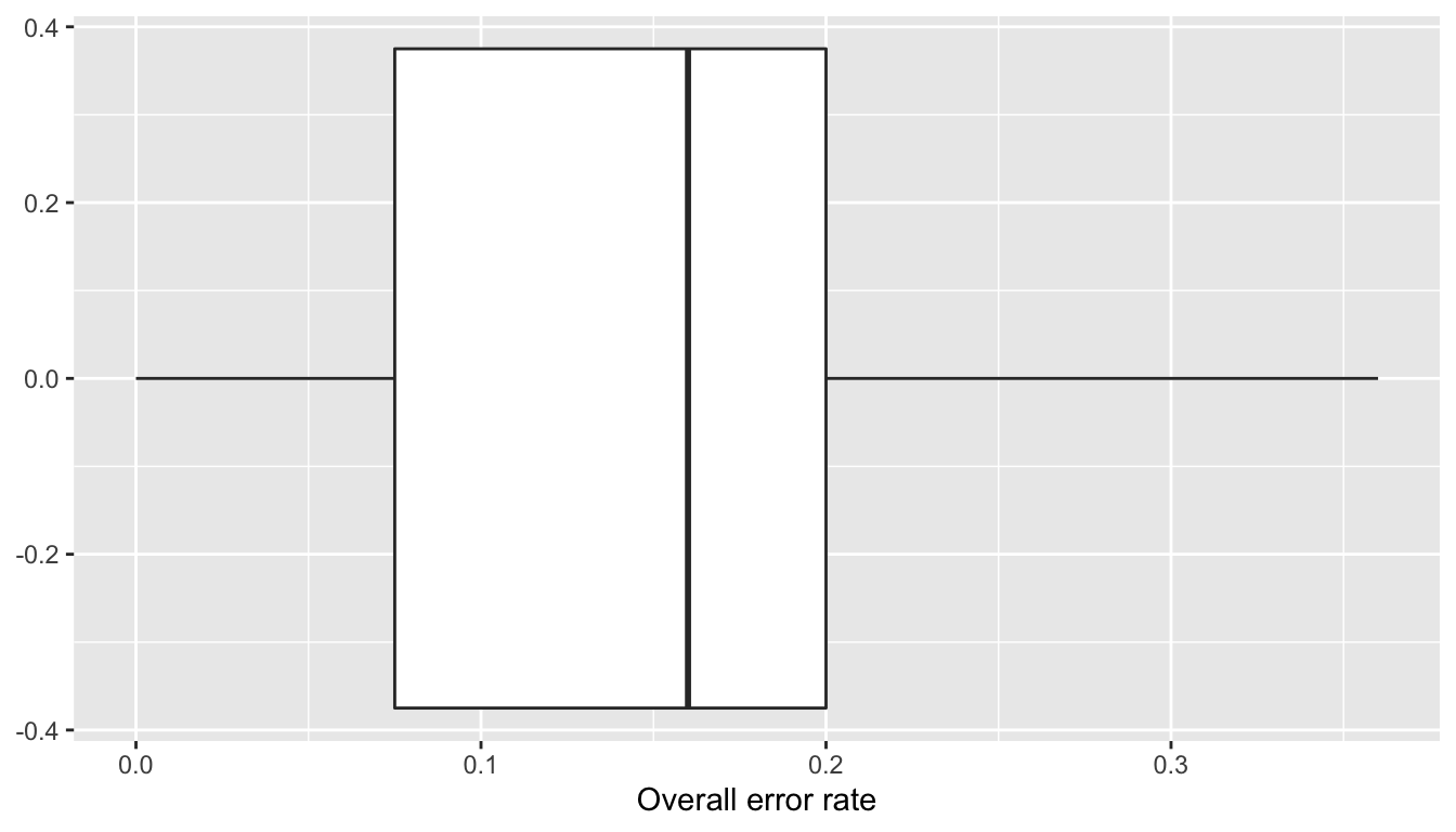
Figure 3.2: Overall error rate over 100 repetitions.
What these error show is that the model is able to “memorize” the data and is able to reproduce not so badly the response variable. We face here some overfitting. With a more flexible model, the error rate could even be equal to zero.
3.1.4 Performances on Unseen Data
Let us go back to our previous regression and let us use our model to make predictions on unseen data.
First, we need some unseen data:
df_test <-
  sample_n(df %>% filter(y == 0), size = n/2, replace= FALSE) %>%
  bind_rows(
    sample_n(df %>% filter(y == 1), size = n/2, replace= FALSE)
  ) %>%
  select(-ID)
The predictions can be obtained as follows:
pred_prob_test <- predict(reg, newdata=df_test)
pred_test <- ifelse(pred_prob_test>.5, 1, 0)
The confusion matrix on these unseen data is obtained with the following instructions:
confusion_matrix_test <- confusion_table(df_test$y, pred_test)
confusion_matrix_test$confusion_matrix_print
## predicted
## observed 0 1
## 0 17 (0.34%) 8 (0.16%)
## 1 16 (0.32%) 9 (0.18%)And here are some metrics obtained thanks to this confusion matrix:
confusion_matrix_test$metrics## $`Erorr rate`
## [1] 0.48
##
## $`True positive rate`
## [1] 0.36
##
## $`False positive rate`
## [1] 0.32
##
## $`True negative rate`
## [1] 0.68
##
## $`False negative rate`
## [1] 0.64
##
## $`Overall error rate`
## [1] 0.48The predictive ability of the model worsened.
Could it be bad luck?
set.seed(123)
# Sample of size 200
n <- 200
df_first_example_2 <-
  sample_n(df %>% filter(y == 0), size = n/2, replace= FALSE) %>%
  bind_rows(
    sample_n(df %>% filter(y == 1), size = n/2, replace= FALSE)
  ) %>%
  select(-ID)
Splitting into train/test to evaluate the capacity of the model to generalise its results on unseen data:
n_train <- round(.8*nrow(df_first_example_2))
ind_train <- sample(1:nrow(df_first_example_2),
                    size = n_train, replace = FALSE)

df_train <- df_first_example_2 %>% slice(ind_train)
df_test <- df_first_example_2 %>% slice(-ind_train)
The dimensions of the training and of the testing datasets:
dim(df_train)## [1] 160 24dim(df_test)## [1] 40 24Let us fit the model on the training set:
reg_train <- glm(y ~ ., data = df_train, family = "binomial")The predictions on the training dataset (in-sample predictions):
pred_train_prob <- predict(reg_train)
pred_train <- ifelse(pred_train_prob>.5, 1, 0)
And the confusion matrix:
confusion_matrix_train <- confusion_table(df_train$y, pred_train)
confusion_matrix_train$confusion_matrix_print
## predicted
## observed 0 1
## 0 68 (0.425%) 14 (0.0875%)
## 1 41 (0.25625%) 37 (0.23125%)confusion_matrix_train$metrics## $`Erorr rate`
## [1] 0.34375
##
## $`True positive rate`
## [1] 0.474359
##
## $`False positive rate`
## [1] 0.1707317
##
## $`True negative rate`
## [1] 0.8292683
##
## $`False negative rate`
## [1] 0.525641
##
## $`Overall error rate`
## [1] 0.34375Let us see our performances on the test set:
pred_test_prob <- predict(reg_train, newdata = df_test)
pred_test <- ifelse(pred_test_prob>.5, 1, 0)
confusion_matrix_test <- confusion_table(df_test$y, pred_test)
confusion_matrix_test$confusion_matrix_print
## predicted
## observed 0 1
## 0 12 (0.3%) 6 (0.15%)
## 1 12 (0.3%) 10 (0.25%)confusion_matrix_test$metrics## $`Erorr rate`
## [1] 0.45
##
## $`True positive rate`
## [1] 0.4545455
##
## $`False positive rate`
## [1] 0.3333333
##
## $`True negative rate`
## [1] 0.6666667
##
## $`False negative rate`
## [1] 0.5454545
##
## $`Overall error rate`
## [1] 0.45We will repeat this procedure 100 times. To make things easier, we can define a function that randomly constitutes a training and a testing datasets from df_first_example_2, fits the model and then returns the confusion matrices as well as the goodness of fit metrics.
train_test_estim <- function(){

  n_train <- round(.8*nrow(df_first_example_2))
  ind_train <-
    sample(1:nrow(df_first_example_2), size = n_train, replace = FALSE)

  df_train <- df_first_example_2 %>% slice(ind_train)
  df_test <- df_first_example_2 %>% slice(-ind_train)

  reg_train <- glm(y ~ ., data = df_train, family = "binomial")
  # Predictions on the train set
  pred_train_prob <- predict(reg_train)
  pred_train <- ifelse(pred_train_prob>.5, 1, 0)
  # On the test set
  pred_test_prob <- predict(reg_train, newdata = df_test)
  pred_test <- ifelse(pred_test_prob>.5, 1, 0)

  # Confusion matrices
  confusion_matrix_train <- confusion_table(df_train$y, pred_train)
  confusion_matrix_test <- confusion_table(df_test$y, pred_test)

  list(confusion_matrix_train = confusion_matrix_train,
       confusion_matrix_test = confusion_matrix_test)

}
The function can be applied over a loop. At each iteration, we can store the results.
results_random_2 <- vector(mode = "list", length = 100)
# pb <- txtProgressBar(min = 1, max = 100, style = 3)
for(i in 1:100){
  results_random_2[[i]] <- train_test_estim()
  # setTxtProgressBar(pb, i)
}
The overall error rates obtained on both sets over the 100 iterations can be obtained as follows:
error_rates_train_2 <-
  map(results_random_2, "confusion_matrix_train") %>%
  map("metrics") %>%
  map_dbl("Overall error rate")

error_rates_test_2 <-
  map(results_random_2, "confusion_matrix_test") %>%
  map("metrics") %>%
map_dbl("Overall error rate")summary(error_rates_train_2)## Min. 1st Qu. Median Mean 3rd Qu. Max.
## 0.2437 0.3047 0.3250 0.3225 0.3438 0.4000summary(error_rates_test_2)## Min. 1st Qu. Median Mean 3rd Qu. Max.
## 0.3000 0.3750 0.4500 0.4427 0.5000 0.6250Let us have a look at these overall error rates on boxplots:
ggplot(data = tibble(error_rate = c(error_rates_train_2,error_rates_test_2),
                     sample = rep(c("Train", "Test"), each = 100))) +
  geom_boxplot(aes(x =error_rate, y = sample)) +
  labs(x = "Overall Error rate", y = "Sample")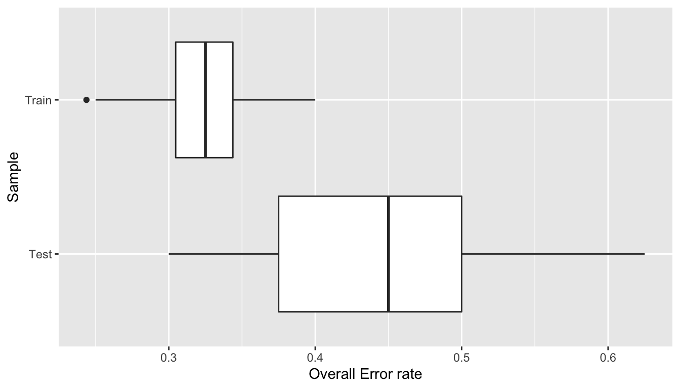
Figure 3.3: Model performance on 100 random draws of the data.
We can see that it was not bad luck in this case. The model tends to make better predictions on the training set and its predictive capacities tend to be worsen on the testing set.
To have an idea of how good the model may perform on unseen data, we can proceed as we just did, but we can also use cross validation.
3.1.5 K-fold Cross Validation
We will use K-fold Cross validation to assess the predictive capacities of the model. We will use a value of \(k=5\).
K-fold Cross Validation
- Consider a dataset with \(n\) training observations. This set of observations can be divided into \(k\) subsets of roughly the same size. Each subset is called a fold.
- In each \(k\)-fold, the fitting procedure is performed on the \(k-1\) folds and evaluated on the \(k\)th fold.
- The error metric is computed at each iteration
- Once each of the \(k\)-fold has served as an evaluation set, we can compute the average of the error metrics (the cross-validation error).
Choice of K
The choice of the number of folds is not straightforward.
- Relatively small values of k lead to larger training samples, which may result in more bias in the estimation of the true surface.
- Relatively high values of k lead to less bias in the estimation of the true surface, but they also lead to a higher variance of the estimated test error.
In the end, it depends on the size and structure of the dataset.
In practice, we often pick k = 3, k = 5 or k = 10.
Here, let us use \(k=5\).
k <- 5We can define a small function that will split a vector into k parts. We will feed this function with the index of rows.
#' Splits a vector into folds
#' @param x vector of observations to be splitted
#' @param k number of desired folds
split_into_folds <- function(x,k)
  split(x, cut(seq_along(x), k, labels = FALSE))
Here is an example of how this function works:
split_into_folds(seq(1, 20), k=3)## $`1`
## [1] 1 2 3 4 5 6 7
##
## $`2`
## [1] 8 9 10 11 12 13
##
## $`3`
## [1] 14 15 16 17 18 19 20Here, we will make a stratified sampling to make sure we end with approximatively the same distribution of the target variable as that of the dataset.
(classes <- unique(df_first_example_2$y))## [1] 0 1folds <- vector(mode = "list", length = length(classes))
for(i in 1:length(classes)){
class <- classes[i]
# row number of obs with target equal to !!class
# shuffle the obs
ind_class <-
sample(which(df_first_example_2$y == class), replace=FALSE)
# split into k folds
folds[[i]] <- split_into_folds(ind_class, k=k)
}
folds <-
map(1:k, ~map(folds, .)) %>%
map(unlist) %>%
map(sample)Here are the row indices in each fold:
folds## [[1]]
## [1] 3 168 139 35 69 1 146 175 160 73 79 60 41 195 18 2 33 108 133
## [20] 138 169 156 131 118 68 123 10 32 50 19 122 47 121 80 162 81 89 101
## [39] 171 141
##
## [[2]]
## [1] 29 20 30 52 116 88 184 183 54 37 77 158 127 113 16 180 173 164 157
## [20] 96 56 57 196 117 92 155 82 40 75 26 153 163 48 192 149 43 14 161
## [39] 190 142
##
## [[3]]
## [1] 93 150 167 194 103 147 191 106 66 84 107 53 176 159 186 177 34 181 87
## [20] 62 13 17 144 135 197 9 200 67 31 193 51 85 4 145 90 70 8 7
## [39] 136 25
##
## [[4]]
## [1] 102 109 22 46 182 63 125 115 104 165 64 98 28 198 5 86 132 114 39
## [20] 119 129 71 45 42 97 94 78 124 61 99 21 111 179 112 23 170 187 83
## [39] 126 178
##
## [[5]]
## [1] 15 137 174 185 120 148 49 55 11 74 44 100 110 27 154 95 189 65 76
## [20] 199 140 143 24 128 152 130 166 151 72 38 58 6 134 59 12 188 91 36
## [39] 105 172We will consider each fold iteratively and make the estimation of the modle on the remaing folds. At each iteration, we will store the overall error rates.
error_rates <- NULLHere is the loop:
for(current_fold in 1:k){
  # All the obs but those of the kth fold
  ind_obs_current <- unlist(folds[-current_fold])
  df_train_current <- df_first_example_2 %>% slice(ind_obs_current)
  df_test_current <- df_first_example_2 %>% slice(-ind_obs_current)

  # Fitting the model
  reg_train <- glm(y ~ ., data = df_train_current, family = "binomial")
  # Predictions on the train set
  pred_train_prob <- predict(reg_train)
  pred_train <- ifelse(pred_train_prob>.5, 1, 0)
  # On the test set
  pred_test_prob <- predict(reg_train, newdata = df_test_current)
  pred_test <- ifelse(pred_test_prob>.5, 1, 0)

  # Confusion matrices
  confusion_matrix_train <- confusion_table(df_train_current$y, pred_train)
  confusion_matrix_test <- confusion_table(df_test_current$y, pred_test)

  error_rate_train <- confusion_matrix_train$metrics$`Overall error rate`
  error_rate_test <- confusion_matrix_test$metrics$`Overall error rate`
  error_rates[[current_fold]] <-
    list(error_rate_train = error_rate_train,
       error_rate_test = error_rate_test)
}
The overall error rate we obtained at each iteration is:
map_dbl(error_rates, "error_rate_train")## [1] 0.33750 0.31250 0.30625 0.34375 0.31250We can calculate the mean of this error:
map_dbl(error_rates, "error_rate_train") %>% mean()## [1] 0.3225And on the test set:
map_dbl(error_rates, "error_rate_test")## [1] 0.400 0.450 0.525 0.475 0.450map_dbl(error_rates, "error_rate_test") %>% mean()## [1] 0.46This mean error gives us a pretty good idea of the average error we will make with unseen data when the model is made into production.
3.1.6 Leave-one-out Cross Validation
Now, let us turn to leave-one-out cross validation.
Leave one out cross validation
- Leave one out cross validation is a \(k\)-fold cross validation where \(k = n\), i.e., the number of folds equals the number of training examples.
- The idea is to leave one observation out and then perform the fitting procedure on all remaining data. - Then, iterate on each data point.
- Each fitting procedure yields an estimation. It is then possible to average the results to get the error metric.
- While this procedure reduces the bias, as it uses all data points, it may be time consuming.
- In addition, the estimations may be influenced by outliers.
This procedure can be implemented as follows:
# Leave one out CV
error_rates_loocv <- NULL

for(i in 1:nrow(df_first_example_2)){
  df_train_current <- df_first_example_2 %>% slice(-i)
  # Single obs:
  df_test_current <- df_first_example_2 %>% slice(i)

  # Fitting the model
  reg_train <- glm(y ~ ., data = df_train_current, family = "binomial")
  # Predictions on the train set
  pred_train_prob <- predict(reg_train)
  pred_train <- ifelse(pred_train_prob>.5, 1, 0)
  # On the test set
  pred_test_prob <- predict(reg_train, newdata = df_test_current)
  pred_test <- ifelse(pred_test_prob>.5, 1, 0)

  avg_error_train <- mean(!pred_train == df_train_current$y)
  avg_error_test <- mean(!pred_test == df_test_current$y)

  error_rates_loocv[[i]] <-
    list(avg_error_train = avg_error_train,
         avg_error_test = avg_error_test)

}
We can have a look at the performances of the model on the training set:
map_dbl(error_rates_loocv, "avg_error_train")## [1] 0.3517588 0.3467337 0.3567839 0.3567839 0.3517588 0.3467337 0.3467337
## [8] 0.3467337 0.3517588 0.3517588 0.3366834 0.3417085 0.3517588 0.3467337
## [15] 0.3467337 0.3366834 0.3417085 0.3517588 0.3417085 0.3417085 0.3266332
## [22] 0.3567839 0.3517588 0.3618090 0.3517588 0.3567839 0.3567839 0.3567839
## [29] 0.3567839 0.3517588 0.3567839 0.3517588 0.3316583 0.3467337 0.3366834
## [36] 0.3517588 0.3517588 0.3517588 0.3517588 0.3567839 0.3467337 0.3517588
## [43] 0.3366834 0.3266332 0.3618090 0.3417085 0.3567839 0.3517588 0.3216080
## [50] 0.3316583 0.3417085 0.3517588 0.3467337 0.3567839 0.3517588 0.3517588
## [57] 0.3567839 0.3517588 0.3165829 0.3467337 0.3467337 0.3417085 0.3517588
## [64] 0.3517588 0.3517588 0.3567839 0.3517588 0.3517588 0.3517588 0.3618090
## [71] 0.3517588 0.3417085 0.3517588 0.3417085 0.3467337 0.3467337 0.3467337
## [78] 0.3467337 0.3618090 0.3567839
## [ reached getOption("max.print") -- omitted 120 entries ]map_dbl(error_rates_loocv, "avg_error_train") %>% mean()## [1] 0.3501005And on the testing set:
map_dbl(error_rates_loocv, "avg_error_test")## [1] 0 1 0 0 0 1 0 0 0 0 1 0 0 0 0 1 0 0 0 1 1 0 0 0 0 0 0 0 0 0 0 0 1 1 1 0 0 0
## [39] 0 0 1 0 1 1 0 0 0 1 1 1 1 0 0 0 0 1 0 0 1 0 0 1 0 0 0 1 0 0 0 1 0 0 1 0 1 0
## [77] 1 0 0 0
## [ reached getOption("max.print") -- omitted 120 entries ]map_dbl(error_rates_loocv, "avg_error_test") %>% mean()## [1] 0.465Once again, this average give us an idea of how good (or bad) our model will perform on unseen data. If the model performs greatly on the training dataset but very poorly on the testing dataset, then we face overfitting.
3.2 Second Example: Selling Price of Cars
In this second example, we will train a machine learning model so that it can predict the selling price of cars. We will use a random forest algorithm to perform this supervised task. We will try different values for one of the hyperparameters of the model, namely the number of variables randomly sampled as candidates at each split (mtry).
In the next hands-on session, we will talk more about random forests. For now, let us just take it as a “black box” for which we need to select a value of one of its hyperparameters. In a nutshell, the higher the value for mtry, the more flexible the model.
The data we will rely on give the selling price of cars (in rupees) and provide details on the characteristics of the car. These were downloaded from Kaggle1 and cleaned (you can download the raw dataset on Kaggle and clean it yourself if you prefer).
The columns of the dataset are the following:
| Variable | Description |
|---|---|
name |
name of the car |
year |
year in which the car was bought |
selling_price |
price the owner wants to sell the car at (in thousand rupees) |
km_driven |
distance completed by the car in km |
fuel |
fuel type of the car |
seller_type |
tells if car is sold by individual or dealer |
transmission |
Gear transmission of the car (Automatic/Manual) |
owner |
number of previous owners |
mileage |
mileage of the car |
engine |
engine capacity of the car |
max_power |
max power of engine |
torque |
torque of the car |
seats |
number of seats in the car |
The data can be loaded as follows:
cars_df <- read_csv("https://egallic.fr/Enseignement/ML/ECB/data/cars.csv")There are 8128 rows and 12 in the dataset.
The target variable is selling_price, i.e., the price of the car:
summary(cars_df$selling_price)## Min. 1st Qu. Median Mean 3rd Qu. Max.
## 30.0 255.0 450.0 638.3 675.0 10000.0sd(cars_df$selling_price)## [1] 806.2534Let us have a quick glance at the correlations for numerical variables:
cars_df %>%
  select(where(is_double)) %>%
  cor(use = "complete.obs")
## year selling_price km_driven mileage engine
## year 1.000000000 0.41230156 -0.42854848 0.3303059 0.0182631
## selling_price 0.412301558 1.00000000 -0.22215848 -0.1198457 0.4556818
## km_driven -0.428548483 -0.22215848 1.00000000 -0.1743984 0.2060307
## mileage 0.330305862 -0.11984571 -0.17439836 1.0000000 -0.5661751
## engine 0.018263100 0.45568180 0.20603073 -0.5661751 1.0000000
## max_power 0.226597796 0.74967378 -0.03815852 -0.3621186 0.7039745
## seats -0.007923033 0.04161669 0.22725939 -0.4462056 0.6111034
## max_power seats
## year 0.22659780 -0.007923033
## selling_price 0.74967378 0.041616694
## km_driven -0.03815852 0.227259388
## mileage -0.36211858 -0.446205571
## engine 0.70397453 0.611103386
## max_power 1.00000000 0.191999183
## seats 0.19199918 1.000000000The proportions of each category for discrete variables can be obtained as follows:
cars_df %>%
  select(selling_price,where(~is.character(.x) | is.factor(.x)), -name) %>%
  pivot_longer(cols = -selling_price) %>%
  group_by(name, value) %>%
  count() %>%
  group_by(name) %>%
  mutate(prop = round(100*n / sum(n), 2)) %>%
  arrange(name, desc(prop))
## # A tibble: 14 × 4
## # Groups: name [4]
## name value n prop
## <chr> <chr> <int> <dbl>
## 1 fuel Diesel 4402 54.2
## 2 fuel Petrol 3631 44.7
## 3 fuel CNG 57 0.7
## 4 fuel LPG 38 0.47
## 5 owner First Owner 5289 65.1
## 6 owner Second Owner 2105 25.9
## 7 owner Third Owner 555 6.83
## 8 owner Fourth & Above Owner 174 2.14
## 9 owner Test Drive Car 5 0.06
## 10 seller_type Individual 6766 83.2
## 11 seller_type Dealer 1126 13.8
## 12 seller_type Trustmark Dealer 236 2.9
## 13 transmission Manual 7078 87.1
## 14 transmission Automatic 1050 12.9Some categories only appear a very restricted number of time. Let us make some changes.
cars_df <-
  cars_df %>%
  mutate(
    fuel = forcats::fct_lump_min(fuel, min = 100, other_level = "Other"),
    owner = forcats::fct_recode(owner, "First Owner" = "Test Drive Car"))
There are some missing values:
cars_df %>%
  summarise(across(everything(), ~sum(is.na(.)))) %>%
  data.frame() %>%
  t()
## [,1]
## name 0
## year 0
## selling_price 0
## km_driven 0
## fuel 0
## seller_type 0
## transmission 0
## owner 0
## mileage 0
## engine 221
## max_power 216
## seats 221Let us use some quick and dirty method here: we will just replace the NA values with the avrage observed in the data. This should require more serious investigation.
Let us also make some feature engineering to augment the dataset, i.e., let us add transformed explanatory variables to the dataset:
cars_df <-
  cars_df %>%
  # replace NA values with average in data
  # (this method is really dirty and should be discussed)
  mutate(
    engine    = replace_na(engine, mean(engine, na.rm=TRUE)),
    max_power = replace_na(max_power, mean(max_power, na.rm=TRUE)),
    seats     = replace_na(seats, mean(seats, na.rm=TRUE)),
    mileage   = ifelse(mileage < 0, yes = NA, no = mileage),
    mileage   = replace_na(mileage, mean(mileage, na.rm=TRUE))
  ) %>%
  mutate(selling_price_log = log(selling_price),
         km_driven_log     = log(km_driven),
         mileage_log       = log(mileage+1),
         engine_log        = log(engine),
         max_power_log     = log(max_power+1))
To fasten the computations in this session, let us only keep 500 observations.
set.seed(456)
cars_df <- cars_df %>% sample_n(1000)
We will use the randomForest() function from {randomForest}. The library thus needs to be loaded.
library(randomForest)Let us split the data into two samples: 80% of the observations in a training sample, and the remaining 20% in a validation sample.
set.seed(456)
n_train <- round(.8*nrow(cars_df))
ind_train <- sample(1:nrow(cars_df), size = n_train, replace = FALSE)
df_train <- cars_df %>% slice(ind_train)
df_valid <- cars_df %>% slice(-ind_train)
Let us check how many observations we have in each samples:
dim(df_train)## [1] 800 17dim(df_valid)## [1] 200 173.2.1 Predicting the Price with a Random Forest
Let us train a random forest on the training data with the following hyperparameters for the algorithm:
ntree=50: we will grow 50 treesmtry=4: at each split in a tree, we will sample only 4 candidate variablesnodesize=10: the Minimum size of terminal nodes is set to 10 (there will be no less than 10 observations in the terminal nodes)
set.seed(456)
mtry <- 4

model_1 <-
  randomForest::randomForest(
    selling_price ~ year + fuel + km_driven +
      seller_type + transmission + owner + mileage +
      engine + max_power + seats,
    data=df_train, importance=TRUE,
    ntree=50, mtry=mtry, nodesize = 10)
The estimated values can be obtained as follows:
predicted_train_1 <- predict(model_1, newdata = df_train)Using those predictions, we can compute the Mean Squared Error (MSE):
resid_train_1 <- df_train$selling_price - predicted_train_1
mse_train_1 <- mean(resid_train_1^2)
mse_train_1
## [1] 16141.57Let us pick another value for mtry a higher value can make the model more flexible and could thus reduce the MSE.
set.seed(456)
mtry <- 7
model_2 <-
  randomForest::randomForest(
    selling_price ~ year + fuel + km_driven +
      seller_type + transmission + owner + mileage +
      engine + max_power + seats,
    data=df_train, importance=TRUE,
    ntree=50, mtry=mtry, nodesize = 10)
Using this second model, let us compute the residuals and then the MSE:
predicted_train_2 <- predict(model_2, newdata = df_train)
resid_train_2     <- df_train$selling_price - predicted_train_2
(mse_train_2 <- mean(resid_train_2^2))
## [1] 16106.57The MSE has indeed decreased. Let us compute the MSE for both models, but this time ondata which were not used to train the model.
predicted_test_1  <- predict(model_1, newdata = df_valid)
predicted_test_2  <- predict(model_2, newdata = df_valid)
resid_test_1      <- df_valid$selling_price - predicted_test_1
resid_test_2      <- df_valid$selling_price - predicted_test_2
mse_test_1 <- mean(resid_test_1^2)
mse_test_2 <- mean(resid_test_2^2)
The MSE computed with the errors made on data never seen by the model are:
mse_test_1 # less flexible model## [1] 21387.4mse_test_2 # more flexible model## [1] 22276.27Let us recall the MSE computed on the train set:
mse_train_1## [1] 16141.57mse_train_2## [1] 16106.57Compared with the less flexible model (the first one), the more flexible model yielded a lower MSE on the training set, but a higher MSE on unseen data. We may suspect some overfitting here.
Let us have a broader look at how the MSE varies as long as we make the model more or less flexible. To do so, we will simply use a loop. At each iteration, we will train the random forest on the same data, but we will make the number of variables randomly sampled as candidates at each split vary.
set.seed(123)
mtry <- c(2,3,4,5,6,7,8)
# pb <- txtProgressBar(min = 1, max = length(mtry), style = 3)
mse <- NULL
for(j in 1:length(mtry)){

  model <-
    randomForest::randomForest(
      selling_price ~ year + fuel + km_driven +
        seller_type + transmission + owner + mileage +
        engine + max_power + seats,
      data=df_train, importance=TRUE,
      ntree=50, mtry=mtry[j], nodesize = 10)

  predicted_train <- predict(model, newdata = df_train)
  predicted_test  <- predict(model, newdata = df_valid)
  resid_train     <- df_train$selling_price - predicted_train
  resid_test      <- df_valid$selling_price - predicted_test

  mse_train <- mean(resid_train^2)
  mse_test  <- mean(resid_test^2)

  mse <- mse %>%
    bind_rows(tibble(mse_train = mse_train, mse_test = mse_test,
                     mtry = mtry[j]))
  # setTxtProgressBar(pb, j)
}mse## # A tibble: 7 × 3
## mse_train mse_test mtry
## <dbl> <dbl> <dbl>
## 1 27188. 30378. 2
## 2 18281. 25414. 3
## 3 16088. 19389. 4
## 4 18224. 27619. 5
## 5 14252. 23608. 6
## 6 14278. 24330. 7
## 7 14439. 24171. 8mse %>%
pivot_longer(cols = -mtry,
names_to = "sample", values_to = "MSE") %>%
mutate(sample = factor(sample, levels = c("mse_train", "mse_test"),
labels = c("Train", "Test"))) %>%
ggplot(data = ., mapping = aes(x = mtry, y = MSE)) +
geom_line(mapping = aes(colour = sample)) +
labs(
x = "Number of variables randomly sampled as candidates at each split",
y = "MSE")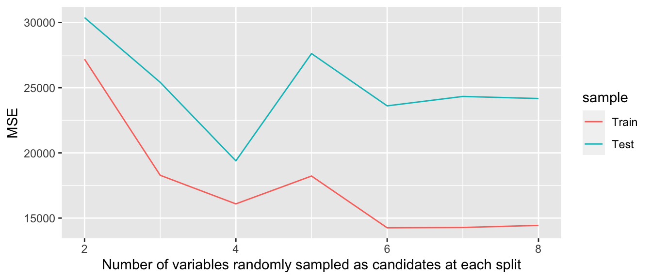
Figure 3.4: Mean Squared Error on Train/Test data..
This graph illustrates multiple things:
- for each value of
mtry, the MSE is relatively higher on the test sample - as long as the hyperparameter
mtryincreases, i.e., as long as the flexibility of the model increases, the mean squared error computed on the training sample diminishes - this is not the case for unseen data: increasing the flexibility of the model may yield better predictions up to a certain flexibility. At some point, however, the model can learn characteristics that are specific to the test sample but which cannot be generalised afterwards: this is overfitting.
3.2.2 Cross-validation to Select the Hyperparameters
In the previous example, we have seen that the predictive capacities of the model are subject to the hyperparameters. This raises the question of the choice of value for these hyperparameters. To do so, a common practice is to perform a grid search and to select the values that yield the best results on unseen data. The performances of the model are assessed using cross-validation. Let us have a look at an example.
Let us only create a very simple grid, in which we will, once again, make a single hyperparameter vary. We will see in the next hands-on session how to perform a slightly more sophisticated grid search.
We will assess the model predictive capacities using k-fold cross-validation, with \(k=5\). The predictive capacities will be evaluated using the MSE.
nb_folds <- 5As in the first example of this notebook, let us define a function that assign the elements of a vector (we will use the row numbers) to one of the k folds.
#' Splits a vector into folds
#' @param x vector of observations to be splitted
#' @param k number of desired folds
split_into_folds <- function(x,k) split(x, cut(seq_along(x), k, labels = FALSE))
Let us assign each observation to a fold:
set.seed(123)
fold_ind <- split_into_folds(sample(1:nrow(df_train)), nb_folds)
We will keep track of the MSE through the iterative process:
mse <- NULLFor each value of the hyperparameter mtry, we will train the random forest \(k\) times. At each of the \(k\) times, the \(k\)-th fold will be left aside to train the machine learning algorithm and will only be used to assess the performances of the model.
mtry <- c(2,3,4,5,6,7,8)
for(j in 1:length(mtry)){
  for(k in 1:nb_folds){
    df_train_current <-
      df_train %>%
      slice(unlist(fold_ind[-k]))

    df_test_current <-
      df_train %>%
      slice(fold_ind[[k]])

    model <-
      randomForest::randomForest(
        selling_price ~ year + fuel + km_driven +
          seller_type + transmission + owner + mileage +
          engine + max_power + seats,
        data=df_train, importance=TRUE,
        ntree=50, mtry=mtry[j], nodesize = 10)

    predicted_train <- predict(model, newdata = df_train_current)
    predicted_test  <- predict(model, newdata = df_test_current)
    resid_train     <- df_train_current$selling_price - predicted_train
    resid_test      <- df_test_current$selling_price - predicted_test

    mse_train <- mean(resid_train^2)
    mse_test  <- mean(resid_test^2)

    mse <- mse %>%
      bind_rows(tibble(mse_train = mse_train, mse_test = mse_test,
                       k = k, mtry = mtry[j]))

  }
}
For each value of mtry, we have obtained \(k\) MSE measures evaluated on the training set and \(k\) MSE measures evaluated on the fold left aside (test set). The average MSE for each value of mtry, both for the train and the test sets can be computed as follows:
mse_summary <-
  mse %>%
  group_by(mtry) %>%
  summarise(
    mse_train = mean(mse_train),
    mse_test = mean(mse_test)
  )
mse_summary
## # A tibble: 7 × 3
## mtry mse_train mse_test
## <dbl> <dbl> <dbl>
## 1 2 26458. 29510.
## 2 3 18376. 17647.
## 3 4 16029. 16240.
## 4 5 15167. 13525.
## 5 6 15704. 18081.
## 6 7 15427. 15310.
## 7 8 14845. 14689.If we only look at the MSE on the train sample, we would be tempted to select a value of 5 for the number of variables to sample from at each split.
mse_summary %>%
  arrange(mse_train)
## # A tibble: 7 × 3
## mtry mse_train mse_test
## <dbl> <dbl> <dbl>
## 1 8 14845. 14689.
## 2 5 15167. 13525.
## 3 7 15427. 15310.
## 4 6 15704. 18081.
## 5 4 16029. 16240.
## 6 3 18376. 17647.
## 7 2 26458. 29510.But looking at the MSE computed on unseen data, a value of 6 may be a better choice.
mse_summary %>%
  arrange(mse_test)
## # A tibble: 7 × 3
## mtry mse_train mse_test
## <dbl> <dbl> <dbl>
## 1 5 15167. 13525.
## 2 8 14845. 14689.
## 3 7 15427. 15310.
## 4 4 16029. 16240.
## 5 3 18376. 17647.
## 6 6 15704. 18081.
## 7 2 26458. 29510.3.3 Third Example: Choice of Lambda in Lasso Regression
Emmanuel Flachaire showed in his slides yesterday that the Lasso regression can be written as follows:
\[\text{minimise}_{\alpha, \boldsymbol{\beta}} \sum_{i=1}^{n} (y_i-\alpha - \boldsymbol{X}_i \boldsymbol{\beta})^2 + \lambda \sum_{j=1}^{p} \lvert \beta_j \rvert.\]
He explained that \(\lambda\) can be selected by cross validation. A pre-built routine in R does it for us (cv.glmnet() from {glmnet}). In this third example, we will use cross validation to select the value for \(\lambda\). We will compare the performances of the model on unseen data by contrasting two situations:
- one in which \(\lambda\) will be selected without cross-validation
- another one in which \(\lambda\) will be selected using cross-validation.
First, let us load the data from {ISLR} (see James et al. (2021), chapter 6):
library(tidyverse)
library(ISLR)
# Removing NA values
Hitters <- na.omit(Hitters)
Let us create the matrix of predictors x and the target variable y (Salary).
x <- model.matrix(Salary ~., Hitters)[,-1]
head(x)
## AtBat Hits HmRun Runs RBI Walks Years CAtBat CHits CHmRun
## -Alan Ashby 315 81 7 24 38 39 14 3449 835 69
## -Alvin Davis 479 130 18 66 72 76 3 1624 457 63
## -Andre Dawson 496 141 20 65 78 37 11 5628 1575 225
## -Andres Galarraga 321 87 10 39 42 30 2 396 101 12
## CRuns CRBI CWalks LeagueN DivisionW PutOuts Assists Errors
## -Alan Ashby 321 414 375 1 1 632 43 10
## -Alvin Davis 224 266 263 0 1 880 82 14
## -Andre Dawson 828 838 354 1 0 200 11 3
## -Andres Galarraga 48 46 33 1 0 805 40 4
## NewLeagueN
## -Alan Ashby 1
## -Alvin Davis 0
## -Andre Dawson 1
## -Andres Galarraga 1
## [ getOption("max.print") est atteint -- 2 lignes omises ]y <- Hitters$Salary
head(y)## [1] 475.0 480.0 500.0 91.5 750.0 70.0We will choose \(\lambda\) by fitting models on a training dataset. The performances of the model will be compared on a validation set:
n_train <- round(.8*nrow(x))
ind_train <- sample(1:nrow(x), size = n_train, replace=FALSE)
x_train <- x[ind_train,]
x_valid <- x[-ind_train,]
y_train <- y[ind_train]
y_valid <- y[-ind_train]
Different values of lambda will be tested:
grid <- 10^seq(2, -2, length = 100)
grid
## [1] 100.00000000 91.11627561 83.02175681 75.64633276 68.92612104
## [6] 62.80291442 57.22367659 52.14008288 47.50810162 43.28761281
## [11] 39.44206059 35.93813664 32.74549163 29.83647240 27.18588243
## [16] 24.77076356 22.57019720 20.56512308 18.73817423 17.07352647
## [21] 15.55676144 14.17474163 12.91549665 11.76811952 10.72267222
## [26] 9.77009957 8.90215085 8.11130831 7.39072203 6.73415066
## [31] 6.13590727 5.59081018 5.09413801 4.64158883 4.22924287
## [36] 3.85352859 3.51119173 3.19926714 2.91505306 2.65608778
## [41] 2.42012826 2.20513074 2.00923300 1.83073828 1.66810054
## [46] 1.51991108 1.38488637 1.26185688 1.14975700 1.04761575
## [51] 0.95454846 0.86974900 0.79248290 0.72208090 0.65793322
## [56] 0.59948425 0.54622772 0.49770236 0.45348785 0.41320124
## [61] 0.37649358 0.34304693 0.31257158 0.28480359 0.25950242
## [66] 0.23644894 0.21544347 0.19630407 0.17886495 0.16297508
## [71] 0.14849683 0.13530478 0.12328467 0.11233240 0.10235310
## [76] 0.09326033 0.08497534 0.07742637 0.07054802 0.06428073
## [ reached getOption("max.print") -- omitted 20 entries ]A function that computes the mean squared error can be defined:
#' Cpmputes the Mean Squared Error
#' @param observed vector of observed data
#' @param predicted vector of predicted values, same length as `observed`
compute_mse <- function(observed, predicted){
  mean((observed - predicted)^2)
}
3.3.1 First Method: Without Cross-Validation
First, we will select a value of \(\lambda\) without using cross-validation.
We need to loop over the different values of \(\lambda\). At each iteration, we will store the value of lambda we used and the computed MSE (calculated on the training set). As we will pick the value of \(\lambda\) based on the performances of the model on already seen data, there is a risk of overfitting.
The list mse_lasso will contain the MSE computed for each value of \(\lambda\).
mse_lasso <- vector(mode = "list", length = length(grid))We need to load {glmnet} to estimate the model:
library(glmnet)And the loop:
for(i in 1:length(grid)){
  lambda <- grid[i]
  lasso_m_current <- glmnet(x = x_train, y = y_train,
                            alpha=1, lambda = lambda, standardize = TRUE)
  predictions_current <- predict(lasso_m_current, newx = x_train)
  mse_lasso[[i]] <- tibble(lambda = lambda, mse = compute_mse(y_train, predictions_current))
}
Let us bind all the tables from the list in a single table, and order the observations by descending values of the MSE:
mse_lasso <-
  bind_rows(mse_lasso) %>%
  arrange(mse)
mse_lasso
## # A tibble: 100 × 2
## lambda mse
## <dbl> <dbl>
## 1 0.0278 102263.
## 2 0.0254 102263.
## 3 0.0231 102263.
## 4 0.0305 102263.
## 5 0.0210 102263.
## 6 0.0192 102263.
## 7 0.0335 102263.
## 8 0.0175 102263.
## 9 0.0159 102263.
## 10 0.0368 102263.
## # … with 90 more rowsThe selected value of \(\lambda\), with such a technique, is the one for which the MSE is the lowest, i.e., the first one in our sorted table:
best_lambda_1 <- mse_lasso$lambda[1]We can plot the MSE as a function of \(\lambda\):
ggplot(data = mse_lasso, mapping = aes(x = lambda, y = mse)) +
  geom_line()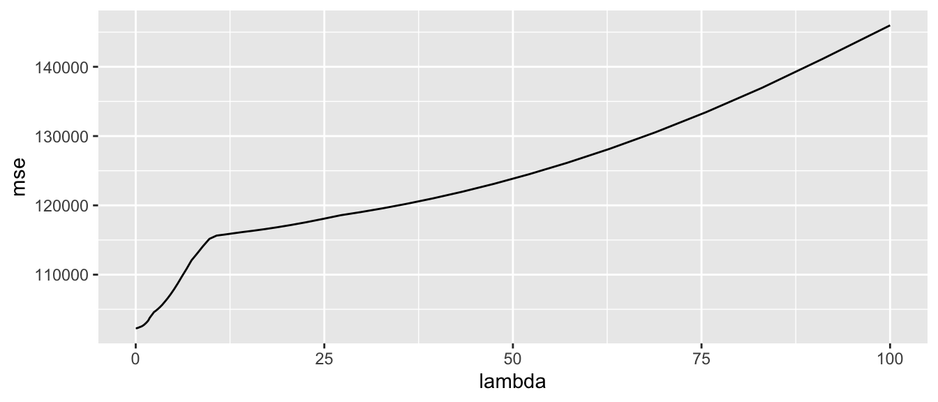
Figure 3.5: Mean Squared Error depending on the value of lambda.
3.3.2 Second Method: With Cross-Validation
To avoid selecting the value of \(\lambda\) by assessing the capabilities of the model to reproduce already seen data, we will use \(k\)-fold cross validation, with \(k=10\).
nb_folds <- 10Let us assign a fold to each data from the training set:
n <- nrow(x_train)
folds <- sample(rep(1:nb_folds, length=n))
As in the first situation, we will use a loop to select the value of \(\lambda\). First, we need to loop on the different folds, and for each fold, we need to train the model on the different values for \(\lambda\) (using a second loop). At each time, we need to store the value of \(\lambda\), the index of the \(k\)-th fold used to compute the MSE, and the computed MSE.
mse <- vector(mode = "list", length = nb_folds)for(k in 1:nb_folds){
ind_current <- folds != k
# Train set
x_train_current <- x_train[ind_current,]
y_train_current <- y_train[ind_current]
# Test set
x_test_current <- x_train[-ind_current,]
y_test_current <- y_train[-ind_current]
# Looping over the values of lambda
mse_fold <- vector(mode = "list", length = length(grid))
for(i in 1:length(grid)){
lambda <- grid[i]
# Estimating on the training set
lasso_m_current <- glmnet(x = x_train_current, y = y_train_current,
alpha=1, lambda = lambda, standardize = TRUE)
# Predictions on the test set
pred_test <- predict(lasso_m_current, x_test_current)
# MSE
mse_test_current <- compute_mse(y_test_current, pred_test)
# Storing the results
mse_fold[[i]] <-
tibble(nb_folds = k, lambda = lambda, mse_test = mse_test_current)
}
mse[[k]] <- bind_rows(mse_fold)
}
mse <- bind_rows(mse)The resulting table looks as follows:
mse## # A tibble: 1,000 × 3
## nb_folds lambda mse_test
## <int> <dbl> <dbl>
## 1 1 100 146138.
## 2 1 91.1 142031.
## 3 1 83.0 137975.
## 4 1 75.6 134597.
## 5 1 68.9 131781.
## 6 1 62.8 129434.
## 7 1 57.2 127478.
## 8 1 52.1 125846.
## 9 1 47.5 124485.
## 10 1 43.3 123348.
## # … with 990 more rowsLet us compute the average and standard deviation of MSE on the k folds:
mse_summary <-
mse %>%
group_by(lambda) %>%
summarise(
mse_sd_test = sd(mse_test),
mse_test = mean(mse_test)
)What is the value of lambda that gives the lowest MSE? To answer this question, we just need to sort the table by descending values of the calculated MSE, and keep the first row.
best_lambda_cv <-
mse_summary %>%
arrange(mse_test) %>%
slice(1)Let us consider the values of \(\lambda\) within a 1-standard error interval:
best_lambda_cv <-
best_lambda_cv %>%
mutate(mse_test_one_sd = mse_test+mse_sd_test)
best_lambda_candidates <-
mse_summary %>%
filter(mse_test <= best_lambda_cv$mse_test_one_sd) %>%
arrange(desc(lambda))
best_lambda_candidates## # A tibble: 61 × 3
## lambda mse_sd_test mse_test
## <dbl> <dbl> <dbl>
## 1 2.66 1303. 106955.
## 2 2.42 1255. 106668.
## 3 2.21 1220. 106446.
## 4 2.01 1228. 106220.
## 5 1.83 1225. 105998.
## 6 1.67 1249. 105797.
## 7 1.52 1279. 105633.
## 8 1.38 1335. 105478.
## 9 1.26 1384. 105363.
## 10 1.15 1444. 105274.
## # … with 51 more rowsAmong the candidates, let us pick the highest:
best_lambda_2 <- best_lambda_candidates$lambda[1]
best_lambda_2## [1] 2.656088Just for the record, we can plot the MSE calculated as a function of \(\lambda\):
mse_summary %>%
ggplot(data = mse_summary, mapping = aes(x = lambda, y = mse_test)) +
geom_line() +
labs(x = "Lambda", y = "MSE")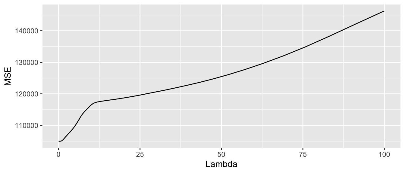
Figure 3.6: Average MSE computed on the left-aside fold.
3.3.3 Comparing the Capacities of the Models on Unseen Data
We have two different values for \(\lambda\):
- one computed without using cross-validation
- another computer with cross-validation
# Model where the value of lambda was selected based on
# the MSE computed using all the observations at hand
lasso_model_1 <-
glmnet(x = x_train, y = y_train,
alpha=1, lambda = best_lambda_1, standardize = TRUE)# Model where the value of lambda was selected using cross-validation
lasso_model_2 <-
glmnet(x = x_train, y = y_train,
alpha=1, lambda = best_lambda_2, standardize = TRUE)Let us predict the values on the validation set for both models:
pred_valid_1 <- predict(lasso_model_1, x_valid)
mse_valid_1 <- compute_mse(y_valid, pred_valid_1)Now we can compute the MSE in both cases:
pred_valid_2 <- predict(lasso_model_2, x_valid)
mse_valid_2 <- compute_mse(y_valid, pred_valid_2)mse_valid_1## [1] 58511.33mse_valid_2## [1] 57736.12One can argue that this result may be due to chance. We can thus make some simulations to reproduce the exact same steps a great number of times.
3.3.4 Repeating the Comparison 100 times
We will repeat the following process 100 times :
- create a training and a validation step
- select \(\lambda\) without cross-validation on training the model on the training sample
- select \(\lambda\) with cross-validation on training the model on the different folds
- fit the models with the two different values of \(\lambda\)
- compute the MSE on the validation set for both models
Please note that this procedure takes a few minutes on a standard computer. We could use parallel computing to fasten it.
nb_repeat <- 100
mse_simulation <- vector(mode = "list", length = nb_repeat)
# pb <- txtProgressBar(min = 1, max = nb_repeat, style = 3)
for(i_repeat in 1:nb_repeat){
# Training and validation sets
n_train <- round(.8*nrow(x))
ind_train <- sample(1:nrow(x), size = n_train, replace=FALSE)
x_train <- x[ind_train,]
x_valid <- x[-ind_train,]
y_train <- y[ind_train]
y_valid <- y[-ind_train]
# 1. Lambda estimated without cross-validation
mse_lasso <- vector(mode = "list", length = length(grid))
for(i in 1:length(grid)){
lambda <- grid[i]
lasso_m_current <- glmnet(x = x_train, y = y_train,
alpha=1, lambda = lambda, standardize = TRUE)
predictions_current <- predict(lasso_m_current, newx = x_train)
mse_lasso[[i]] <-
tibble(lambda = lambda,
mse = compute_mse(y_train, predictions_current))
}
mse_lasso <-
bind_rows(mse_lasso) %>%
arrange(mse)
best_lambda_1 <- mse_lasso$lambda[1]
#2. Lambda estimated with cross-validation
folds <- sample(rep(1:nb_folds, length=n))
mse <- vector(mode = "list", length = nb_folds)
for(k in 1:nb_folds){
  ind_current <- folds != k

  # Train set
  x_train_current <- x_train[ind_current,]
  y_train_current <- y_train[ind_current]
  # Test set
  x_test_current <- x_train[-ind_current,]
  y_test_current <- y_train[-ind_current]

  # Looping over the values of lambda
  mse_fold <- vector(mode = "list", length = length(grid))
  for(i in 1:length(grid)){
    lambda <- grid[i]
    # Estimating on the training set
    lasso_m_current <- glmnet(x = x_train_current, y = y_train_current,
                              alpha=1, lambda = lambda, standardize = TRUE)
    # Predictions on the test set
    pred_test <- predict(lasso_m_current, x_test_current)
    # MSE
    mse_test_current <- compute_mse(y_test_current, pred_test)

    # Storing the results
    mse_fold[[i]] <-
      tibble(nb_folds = k, lambda = lambda, mse_test = mse_test_current)
  }
  mse[[k]] <- bind_rows(mse_fold)

}
mse <- bind_rows(mse)
# Compute the average and standard deviation of MSE on the k folds
mse_summary <-
  mse %>%
  group_by(lambda) %>%
  summarise(
    mse_sd_test = sd(mse_test),
    mse_test = mean(mse_test)
  )
# What is the value of lambda that gives the lowest MSE?
best_lambda_cv <-
  mse_summary %>%
  arrange(mse_test) %>%
slice(1) %>%
mutate(mse_test_one_sd = mse_test+mse_sd_test)
# Lambdas within 1 standard error
best_lambda_candidates <-
mse_summary %>%
filter(mse_test <= best_lambda_cv$mse_test_one_sd) %>%
arrange(desc(lambda))
# Among the candidates, let us pick the highest
best_lambda_2 <- best_lambda_candidates$lambda[1]
# 3. Performance on the validation set
# Model where the value of lambda was selected based on
# the MSE computed using all the observations at hand
lasso_model_1 <-
  glmnet(x = x_train, y = y_train,
         alpha=1, lambda = best_lambda_1, standardize = TRUE)
# Model where the value of lambda was selected using cross-validation
lasso_model_2 <-
  glmnet(x = x_train, y = y_train,
         alpha=1, lambda = best_lambda_2, standardize = TRUE)
# Predictions:
pred_valid_1 <- predict(lasso_model_1, x_valid)
mse_valid_1 <- compute_mse(y_valid, pred_valid_1)
pred_valid_2 <- predict(lasso_model_2, x_valid)
mse_valid_2 <- compute_mse(y_valid, pred_valid_2)
mse_simulation[[i_repeat]] <-
tibble(i = i_repeat, mse_valid_1 = mse_valid_1, mse_valid_2)
# setTxtProgressBar(pb, i_repeat)
}
mse_simulation <- bind_rows(mse_simulation)We end up with a table with the MSE for the 100 simulations:
mse_simulation## # A tibble: 100 × 3
## i mse_valid_1 mse_valid_2
## <int> <dbl> <dbl>
## 1 1 153647. 131441.
## 2 2 137854. 116347.
## 3 3 222221. 220751.
## 4 4 76973. 79704.
## 5 5 55429. 50502.
## 6 6 105757. 91559.
## 7 7 103680. 101132.
## 8 8 164501. 148567.
## 9 9 129571. 125734.
## 10 10 137936. 149992.
## # … with 90 more rowsLet us look at how many replications yielded lower MSE on the validation set when \(\lambda\) was selected by cross-validation:
mse_simulation %>%
  mutate(lower_with_cv = mse_valid_2 < mse_valid_1) %>%
  group_by(lower_with_cv) %>%
  count()
## # A tibble: 2 × 2
## # Groups: lower_with_cv [2]
## lower_with_cv n
## <lgl> <int>
## 1 FALSE 29
## 2 TRUE 71And we can also compute some descriptive statistics:
mse_simulation %>%
  pivot_longer(cols = -i) %>%
  group_by(name) %>%
  summarise(mean = mean(value),
            sd = sd(value),
            q_1 = quantile(value, probs = .25),
            med = quantile(value, probs = .5),
            q_3 = quantile(value, probs = .75)
            )
## # A tibble: 2 × 6
## name mean sd q_1 med q_3
## <chr> <dbl> <dbl> <dbl> <dbl> <dbl>
## 1 mse_valid_1 130271. 43112. 100508. 134385. 157273.
## 2 mse_valid_2 126686. 43244. 93671. 123173. 156620.And lastly, we can look at the distribution of the MSE with boxplots:
mse_simulation %>%
  pivot_longer(cols = -i, names_to = "sample", values_to = "MSE") %>%
  mutate(sample = factor(sample, levels = c("mse_valid_1", "mse_valid_2"),
                         labels = c("Without CV", "With CV"))) %>%
  ggplot(data = ., mapping = aes(y = MSE)) +
  geom_boxplot(mapping = aes(fill = sample)) +
  scale_fill_discrete("Choice of lambda")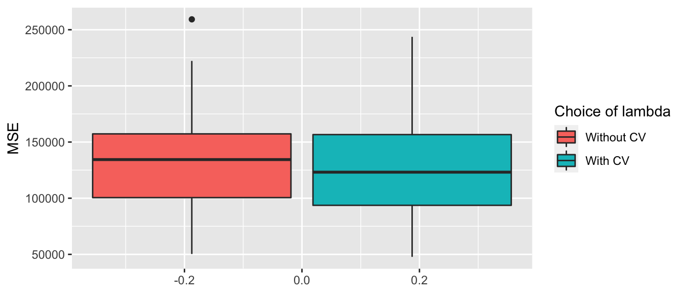
Figure 3.7: MSE on the replications depending on how lambda was selected.