12  Local Projections with Quarterly Data

\[ \definecolor{bayesred}{RGB}{147, 30, 24} \definecolor{bayesblue}{RGB}{32, 35, 91} \definecolor{bayesorange}{RGB}{218, 120, 1} \definecolor{grey}{RGB}{128, 128, 128} \definecolor{couleur1}{RGB}{0,163,137} \definecolor{couleur2}{RGB}{255,124,0} \definecolor{couleur3}{RGB}{0, 110, 158} \definecolor{coul1}{RGB}{255,37,0} \definecolor{coul2}{RGB}{242,173,0} \definecolor{col_neg}{RGB}{155, 191, 221} \definecolor{col_pos}{RGB}{255, 128, 106} \definecolor{wongBlack}{RGB}{0,0,0} \definecolor{wongLightBlue}{RGB}{86, 180, 233} \definecolor{wongGold}{RGB}{230, 159, 0} \definecolor{wongGreen}{RGB}{0, 158, 115} \definecolor{wongYellow}{RGB}{240, 228, 66} \definecolor{wongBlue}{RGB}{0, 114, 178} \definecolor{wongOrange}{RGB}{213, 94, 0} \definecolor{wongPurple}{RGB}{204, 121, 167} \definecolor{IBMPurple}{RGB}{120, 94, 240} \definecolor{IBMMagenta}{RGB}{220, 38, 127} \]

This chapter uses Jordà (2005) Local Projection framework to measure how sensitive agricultural output is to exogenous changes in the weather. Instead of using monthly data as in Chapter 7, we use here quarterly data.

library(tidyverse)

── Attaching core tidyverse packages ──────────────────────── tidyverse 2.0.0 ──
✔ dplyr     1.1.4     ✔ readr     2.1.4
✔ forcats   1.0.0     ✔ stringr   1.5.0
✔ ggplot2   3.4.4     ✔ tibble    3.2.1
✔ lubridate 1.9.3     ✔ tidyr     1.3.0
✔ purrr     1.0.2     
── Conflicts ────────────────────────────────────────── tidyverse_conflicts() ──
✖ dplyr::filter() masks stats::filter()
✖ dplyr::lag()    masks stats::lag()
ℹ Use the conflicted package (<http://conflicted.r-lib.org/>) to force all conflicts to become errors

library(fastDummies)

The data can be loaded (see Chapter 11)

load("../data/output/df_lp_quarter.rda")
df

# A tibble: 4,080 × 29
   product_eng region_id  year quarter  y_new     y region   product Value_prod
   <chr>       <fct>     <dbl>   <dbl>  <dbl> <dbl> <chr>    <chr>        <dbl>
 1 Cassava     1          2001       1 15374. 1.27  AMAZONAS YUCA        15374.
 2 Cassava     1          2001       2 16300. 1.12  AMAZONAS YUCA        16300.
 3 Cassava     1          2001       3 17152. 1.24  AMAZONAS YUCA        17152.
 4 Cassava     1          2001       4 18010. 1.36  AMAZONAS YUCA        18010.
 5 Cassava     1          2002       1 16763  1.13  AMAZONAS YUCA        16763 
 6 Cassava     1          2002       2 18472  0.983 AMAZONAS YUCA        18472 
 7 Cassava     1          2002       3 20775  1.13  AMAZONAS YUCA        20775 
 8 Cassava     1          2002       4 19990  1.21  AMAZONAS YUCA        19990 
 9 Cassava     1          2003       1 16591  0.964 AMAZONAS YUCA        16591 
10 Cassava     1          2003       2 19460  0.833 AMAZONAS YUCA        19460 
# ℹ 4,070 more rows
# ℹ 20 more variables: rer_hp <dbl>, r_hp <dbl>, pi <dbl>, ind_prod <dbl>,
#   price_int <dbl>, int_price_inf <dbl>, temp_min <dbl>, temp_max <dbl>,
#   temp_mean <dbl>, precip_sum <dbl>, perc_gamma_precip <dbl>,
#   temp_min_dev <dbl>, temp_max_dev <dbl>, temp_mean_dev <dbl>,
#   precip_sum_dev <dbl>, ONI <dbl>, temp_min_dev_ENSO <dbl>,
#   temp_max_dev_ENSO <dbl>, temp_mean_dev_ENSO <dbl>, …

Some packages are needed, make sure that they are installed.

# install.packages("fastDummies")
# install.packages("imputeTS")
# install.packages("ggh4x")
# install.packages("mFilter")
# install.packages("pbapply")
# install.packages("latex2exp")
# install.packages("sandwich")

We load some useful functions:

# Functions useful to shape the data for local projections
source("../weatherperu/R/format_data-quarter.R")

# Load function in utils
source("../weatherperu/R/utils.R")

# Load detrending functions
source("../weatherperu/R/detrending-quarter.R")

12.1 Linear Local Projections

In this section, we focus on estimating the Local Projections (Jordà 2005) to quantify the impact of weather on agricultural production. We utilize panel data, similar to the approach used in the study by Acevedo et al. (2020), and independently estimate models for each specific crop.

For a particular crop denoted as \(c\), the model can be expressed as follows: \[ \begin{aligned} \underbrace{y_{c,i,{\color{wongGold}t+h}}}_{\text{Production}} = & \underbrace{\alpha_{c,i,h}}_{\text{reg. fixed effect}} + {\color{wongOrange}\beta_{c,{\color{wongGold}h}}^{{\color{wongPurple}T}}} {\color{wongPurple}{T_{i,{\color{wongGold}t}}}} + {\color{wongOrange}\beta_{c,{\color{wongGold}h}}^{{\color{wongPurple}P}}} {\color{wongPurple}P_{i,{\color{wongGold}t}}}\\ &+\delta_{c,i,h}\underbrace{X_{t}}_{\text{controls}}+\varepsilon_{c,i,t+h} \end{aligned} \tag{12.1}\]

Here, \(i\) represents the region, \(t\) represents the time, and \(h\) represents the horizon. The primary focus lies on estimating the coefficients associated with temperature and precipitation for different time horizons \(\color{wongGold}h=\{0,1,...,T_{c}\}\)

12.1.1 Functions

To estimate the models, we develop a function, get_data_lp(), that generates the endogenous variable and the regressors for a specific crop, considering a given time horizon. This function is designed to return a list where each element represents the dataset that will be utilized for estimating the model corresponding to a specific time horizon.

When we call the get_data_lp() function, we check for missing values in the weather data. If missing values are present for a specific region and crop, we keep only the longest consecutive sequence without missing values. To achieve this, we use the two functions defined previously: get_index_longest_non_na() and keep_values_longest_non_na().

#' Get the data in a table for the local projections, for a specific crop
#'
#' @param df original dataset
#' @param horizons number of horizons
#' @param y_name name of the exogenous variable
#' @param group_name name of the group variable
#' @param crop_name name of the crop to focus on
#' @param control_names vector of names of the control variables
#' @param weather_names vector of names of the weather variables
#' @param add_quarter_fe should columns with quarter dummy variables be added?
#'   Default to `TRUE`
#' @param share_geo vector of names of the variables that contain the share of
#'   each type of geographical pattern. By default `NULL`: no share used
#' @param transition_name name of the variable used to define the transition to
#'   the two states. By default `NULL`
#' @param transition_method if transition function, name of the method to use:
#'   `logistic` or `normal` (default to `NULL`, i.e., no transition)
#' @param state_names name of the two states in a vector of characters (only if
#'   `transition_name` is not `NULL`). First period corresponds to mapped values
#'   of `transition_name` close to 0, which is for large positive values of
#'   `transition_name`
#' @param gamma logistic growth rate (default to 3, only used if
#'   `transition_name` is not `NULL`)
#' @param other_var_to_keep vector of names of other variables to keep (default
#'   to `NULL`: no additional vairable kept)
#' @export
#' @importFrom dplyr filter select mutate sym group_by across rowwise arrange
#'   slice lead ends_with
#' @importFrom fastDummies dummy_cols
#' @importFrom stringr str_c str_detect
get_data_lp <- function(df,
                        horizons,
                        y_name,
                        group_name,
                        crop_name,
                        control_names,
                        weather_names,
                        add_quarter_fe = TRUE,
                        share_geo = NULL,
                        transition_name = NULL,
                        transition_method = NULL,
                        state_names = c("planted", "harvested"),
                        gamma = 3,
                        other_var_to_keep = NULL) {

  if (!is.null(share_geo) & !is.null(transition_name)) {
    stop("You can only use one between share_geo and transition_name")
  }

  # Init empty object to return: list of length horizons
  df_horizons <- vector(mode = "list", length = horizons + 1)

  # Keep only the variables needed
  df_focus <-
    df |>
    filter(product_eng == !!crop_name) |>
    select(
      !!y_name,
      !!group_name,
      year,
      quarter,
      product_eng,
      !!!control_names,
      !!!weather_names,
      !!!share_geo,
      !!transition_name,
      !!other_var_to_keep
    ) |>
    mutate(
      !!group_name := factor(!!sym(group_name))
    )

  # Quarter dummy fixed-effects
  if (add_quarter_fe) {
    df_focus <- df_focus |>
      # mutate(
      #   quarter = as.character(lubridate::quarter(date))
      # ) |>
      dummy_cols(select_columns = "quarter", remove_first_dummy = FALSE)
  }


  # For each region, only keep the longest sequence of non NA values found in
  # the weather variables
  df_focus <-
    df_focus |>
    group_by(region_id) |>
    mutate(
      across(
        .cols  = !!weather_names,
        .fns   = keep_values_longest_non_na,
        .names = "{.col}_keep"
      )
    ) |>
    rowwise() |>
    mutate(keep_cols = all(across(ends_with("_keep")))) |>
    ungroup() |>
    filter(keep_cols) |>
    select(-keep_cols, -!!paste0(weather_names, "_keep"))

  if (!is.null(share_geo)) {
    # For each geographical type, multiply the weather variables by the share
    # that the geo. type represents
    for(share_geo_type in share_geo) {
      df_focus <-
        df_focus |>
        mutate(
          across(
            .cols  = !!weather_names,
            .fns   = ~ .x * !!sym(share_geo_type),
            .names = str_c("{.col}_", share_geo_type)
          )
        )
    }
  }

  if (!is.null(transition_name)) {

    state_1_name <- state_names[1]
    state_2_name <- state_names[2]

    if (transition_method == "logistic") {
      df_focus <-
        df_focus |>
        mutate(
          fz = logist(!!sym(transition_name), gamma = gamma)
        )
    } else if (transition_method == "normal") {
      df_focus <-
        df_focus |>
        mutate(
          fz = pnorm(-!!sym(transition_name))
        )
    } else {
      stop("transition method must be either \"losistic\" or \"normal\"")
    }
    df_focus <- df_focus |>
      dummy_cols(group_name, remove_first_dummy = FALSE)

    ind_dummies_group <- str_detect(colnames(df_focus), str_c(group_name, "_"))
    dummies_group_name <- colnames(df_focus)[ind_dummies_group]

    if (add_quarter_fe) {
      ind_dummies_quarter <- str_detect(colnames(df_focus), "^quarter_")
      dummies_quarter_name <- colnames(df_focus)[ind_dummies_quarter]
      dummies_group_name <- c(dummies_group_name, dummies_quarter_name)
    }

    df_focus <-
      df_focus |>
      mutate(
        # First regime:
        across(
          .cols  = c(!!!control_names, !!!weather_names, !!!dummies_group_name),
          .fns   = list(
            state_1_name = ~ (1 - fz) * .x,
            state_2_name = ~ fz * .x
          ),
          .names = "{fn}_{col}"
        )
      ) |>
      rename_with(
        .fn = ~str_replace(string = .x, pattern = "state_1_name", replacement = state_1_name),
        .cols = starts_with("state_1_name")
      ) |>
      rename_with(
        .fn = ~str_replace(string = .x, pattern = "state_2_name", replacement = state_2_name),
        .cols = starts_with("state_2_name")
      )
  } else {
    df_focus <-
      df_focus |>
      dummy_cols(group_name, remove_first_dummy = FALSE)
  }


  # Prepare the values for y at t+h
  for (h in 0:horizons) {
    df_horizons[[h+1]] <-
      df_focus |>
      group_by(!!sym(group_name)) |>
      arrange(year, quarter) |>
      mutate(y_lead = dplyr::lead(!!sym(y_name), n = h)) |>
      slice(1:(n()-h))
  }
  names(df_horizons) <- 0:horizons
  df_horizons
}

Following the data preparation step, we proceed to define a function, estimate_linear_lp() that performs the estimation of models for all time horizons. This function utilizes the datasets obtained through the get_data_lp() function.

#' Estimate Local Projections
#'
#' @param df original dataset
#' @param horizons number of horizons
#' @param y_name name of the exogenous variable
#' @param group_name name of the group variable
#' @param crop_name name of the crop to focus on
#' @param control_names vector of names of the control variables
#' @param weather_names vector of names of the weather variables
#' @param add_quarter_fe should columns with quarter dummy variables be added?
#'   Default to `TRUE`
#' @param add_intercept should an intercept we added to the regressions?
#'   (default to `FALSE`)
#' @param share_geo vector of names of the variables that contain the share of
#'   each type of geographical pattern. By default `NULL`: no share used
#' @param std type of standard error (`"NW"` for Newey-West, `"Cluster"`,
#'   `"Standard"` otherwise)
#' @param transition_name name of the variable used to define the transition to
#'   the two states. By default `NULL`
#' @param transition_method if transition function, name of the method to use:
#'   `logistic` or `normal` (default to `NULL`, i.e., no transition)
#' @param state_names name of the two states in a vector of characters (only if
#'   `transition_name` is not `NULL`). First period corresponds to mapped values
#'   of `transition_name` close to 0, which is for large positive values of
#'   `transition_name`
#' @param gamma logistic growth rate (default to 3, only used if
#'   `transition_name` is not `NULL`)
#' @param other_var_to_keep vector of names of other variables to keep in the
#'   returned dataset (default to `NULL`: no additional vairable kept)
#' @export
#' @importFrom dplyr mutate sym ungroup summarise across left_join
#' @importFrom stringr str_c str_detect
#' @importFrom purrr map map_dbl list_rbind
#' @importFrom tibble enframe
#' @importFrom tidyr pivot_longer
#' @importFrom sandwich NeweyWest
#' @importFrom stats sd model.matrix nobs residuals lm coef
estimate_linear_lp <- function(df,
                              horizons,
                              y_name,
                              group_name,
                              crop_name,
                              control_names,
                              weather_names,
                              add_quarter_fe = TRUE,
                              add_intercept = FALSE,
                              share_geo = NULL,
                              transition_name = NULL,
                              transition_method = NULL,
                              state_names = c("planted", "harvested"),
                              gamma = 3,
                              std = c("nw", "cluster", "standard"),
                              other_var_to_keep = NULL) {

  # Format the dataset
  data_lp <-
    get_data_lp(
      df = df,
      horizons = horizons,
      y_name = y_name,
      group_name = group_name,
      crop_name = crop_name,
      control_names = control_names,
      weather_names = weather_names,
      share_geo = share_geo,
      transition_name = transition_name,
      transition_method = transition_method,
      state_names = state_names,
      gamma = gamma,
      other_var_to_keep = other_var_to_keep
    )

  # Recode levels for the groups
  for(h in 0:horizons){
    data_lp[[h + 1]] <-
      data_lp[[h + 1]] |>
      mutate(
        !!group_name := as.factor(as.character(!!sym(group_name)))
      )
  }

  control_names_full <- control_names
  weather_names_full <- weather_names
  ind_names_groups <- str_detect(
    colnames(data_lp[[1]]), str_c("^", group_name, "_")
  )
  group_names_full <- colnames(data_lp[[1]])[ind_names_groups]

  if (!is.null(share_geo)) {
    # Name of the weather variables
    weather_names_full <- paste(
      rep(weather_names, each = length(share_geo)),
      share_geo,
      sep = "_"
    )
  }

  if (!is.null(transition_name)) {

    state_1_name <- str_c(state_names[1], "_")
    state_2_name <- str_c(state_names[2], "_")

    # Name of the variables
    weather_names_full <- str_c(
      rep(
        c(state_1_name, state_2_name),
        each = length(weather_names)
      ),
      rep(weather_names, 2)
    )
    control_names_full <- str_c(
      rep(
        c(state_1_name, state_2_name),
        each = length(control_names)
      ),
      rep(control_names, 2)
    )
    ind_names_groups <- str_detect(
      colnames(data_lp[[1]]),
      str_c("(^", state_1_name, "|", state_2_name, ")", group_name, "_")
    )
    group_names_full <- colnames(data_lp[[1]])[ind_names_groups]
  }

  # Observed standard deviations in the data
  sd_weather_shock <-
    map(
      .x = data_lp,
      .f = ~ungroup(.x) |>
        summarise(
          across(
            .cols  = c(!!control_names_full, !!weather_names_full, !!share_geo),
            .fns   = sd
          )
        )
    ) |>
    list_rbind(names_to = "horizon") |>
    pivot_longer(cols = -horizon, names_to = "name", values_to = "std_shock") |>
    mutate(horizon = as.numeric(horizon))

  # Observed median value in the data
  median_weather_shock <-
    map(
      .x = data_lp,
      .f = ~ungroup(.x) |>
        summarise(
          across(
            .cols  = c(!!control_names_full, !!weather_names_full, !!share_geo),
            .fns   = ~quantile(.x, probs = .5)
          )
        )
    ) |>
    list_rbind(names_to = "horizon") |>
    pivot_longer(cols = -horizon, names_to = "name", values_to = "median_shock") |>
    mutate(horizon = as.numeric(horizon))

  # Observed quantile of order 0.05 value in the data
  q05_weather_shock <-
    map(
      .x = data_lp,
      .f = ~ungroup(.x) |>
        summarise(
          across(
            .cols  = c(!!control_names_full, !!weather_names_full, !!share_geo),
            .fns   = ~quantile(.x, probs = .05)
          )
        )
    ) |>
    list_rbind(names_to = "horizon") |>
    pivot_longer(cols = -horizon, names_to = "name", values_to = "q05_shock") |>
    mutate(horizon = as.numeric(horizon))

  # Observed quantile of order 0.95 value in the data
  q95_weather_shock <-
    map(
      .x = data_lp,
      .f = ~ungroup(.x) |>
        summarise(
          across(
            .cols  = c(!!control_names_full, !!weather_names_full, !!share_geo),
            .fns   = ~quantile(.x, probs = .95)
          )
        )
    ) |>
    list_rbind(names_to = "horizon") |>
    pivot_longer(cols = -horizon, names_to = "name", values_to = "q95_shock") |>
    mutate(horizon = as.numeric(horizon))


  # Formula for the regressions
  formula_lp <- paste0(
    "y_lead",
    " ~ -1+",
    # " ~ 1+", # intercept
    paste(weather_names_full, collapse = " + "),
    " + ",
    paste(control_names_full, collapse = " + "),
    " + ",
    ifelse(
      add_intercept,
      # removing last group
      yes = paste(group_names_full[-length(group_names_full)], collapse = " + "),
      # keeping last group
      no = paste(group_names_full, collapse = " + ")
    )
  )

  if (add_quarter_fe) {
    formula_lp <- paste0(
      formula_lp, " + ", paste(paste0("quarter_", 1:11), collapse = " + ")
    )
  }

  # Regressions
  reg_lp <- map(data_lp, ~ lm(formula = formula_lp, data = .))

  # Standard error of the residuals
  sig_ols <- map_dbl(.x = reg_lp, .f = ~sd(.x$residuals))

  log_likelihood <- map_dbl(
    .x = reg_lp,
    .f = function(reg) {
      err_x <- reg$residuals
      sig_ols <- sd(err_x)
      sum(log(1 / sqrt(2 * pi * sig_ols^2) * exp(-err_x^2 / (2 * sig_ols^2))))
    }
  )

  mse <- map_dbl(
    .x = reg_lp,
    .f = function(reg) {
      err_x <- reg$residuals
      mean(err_x^2)
    }
  )

  coefs <- map(
    reg_lp,
    ~ enframe(coef(.))
  ) |>
    list_rbind(names_to = "horizon")

  if (std == "nw") {
    # Newey-West
    cov_nw_pw <- map(
      reg_lp,
      ~ sandwich::NeweyWest(.x, lag = 1, prewhite = FALSE)
    )
    se_df <- map(
      cov_nw_pw,
      ~ enframe(sqrt(diag(.)), value = "std")
    ) |>
      list_rbind(names_to = "horizon")
  } else if (std == "Cluster") {
    cl_std <- vector(mode = "list", length = horizons + 1)
    names(cl_std) <- 0:horizons
    for (h in 0:horizons) {
      ind_NA_coef <- which(is.na(reg_lp[[h + 1]]$coefficients))
      X <- model.matrix(reg_lp[[h + 1]])
      if (length(ind_NA_coef) > 1) {
        X <- X[, -ind_NA_coef]
      }

      errx <- residuals(reg_lp[[h + 1]])
      omega <- 0
      m_clust <- ifelse(
        add_intercept,
        yes = length(group_names_full[-length(group_names_full)]),
        no = length(group_names_full)
      )
      n_clust <- length(errx)
      k_clust <- ncol(X)
      for (ri in 1:m_clust) {
        # Identify id row within the cluster
        idx <- which(X[, group_names_full[ri]] == 1)
        omega <- omega + t(X[idx, ]) %*% errx[idx] %*% t(errx[idx]) %*% X[idx, ]
      }

      omega <- m_clust / (m_clust - 1) * (n_clust - 1) / (n_clust - k_clust) * omega
      t1 <- solve(t(X) %*% X)
      colSums(t1)
      v_cluster <- t1 %*% omega %*% t1
      cl_std[[h + 1]] <- sqrt(diag(v_cluster))
      names(cl_std[[h + 1]]) <- colnames(omega)

    }
    se_df <-
      map(cl_std, ~enframe(., value = "std")) |>
      list_rbind(names_to = "horizon")
  } else {
    se_df <- map(
      reg_lp,
      ~ enframe(sqrt(diag(vcov(.))), value = "std")
    ) |>
      list_rbind(names_to = "horizon")
  }

  coefs <-
    coefs |>
    left_join(se_df, by = c("horizon", "name")) |>
    mutate(
      crop = crop_name,
      horizon = as.numeric(horizon)
    ) |>
    left_join(sd_weather_shock, by = c("horizon", "name")) |>
    left_join(median_weather_shock, by = c("horizon", "name")) |>
    left_join(q05_weather_shock, by = c("horizon", "name")) |>
    left_join(q95_weather_shock, by = c("horizon", "name"))

  list(
    # reg_lp = reg_lp,
    coefs = coefs,
    horizons = horizons,
    log_likelihood = log_likelihood,
    mse = mse,
    crop_name = crop_name,
    data_lp = data_lp
  )
}

Note

The get_data_lp() function is defined in the R script saved here: /weatherperu/R/format_data-quarter.R. The estimation function, estimate_linear_lp(), is defined in the R script saved here: /weatherperu/R/estimations-quarter.R.

source("../weatherperu/R/estimations-quarter.R")

12.1.2 Estimation

To loop over the different crops, we can utilize the map() function. This function enables us to apply the estimate_linear_lp() function to each crop iteratively, facilitating the estimation process.

crops <- df$product_eng |> unique()
weather_variables <- c("temp_max_dev", "precip_sum_dev")
control_variables <- c(
  "rer_hp", "r_hp", "pi", "ind_prod", "ONI", "int_price_inf"
)

resul_lp_quarter <- map(
  crops, ~ estimate_linear_lp(
    df,
    horizons = 4,
    y_name = "y",
    group_name = "region_id",
    add_quarter_fe = FALSE,
    add_intercept = FALSE,
    crop_name = .x,
    control_names = control_variables,
    weather_names = weather_variables,
    std = "Cluster",
    other_var_to_keep = "y_new"
  )
)

12.1.3 Results

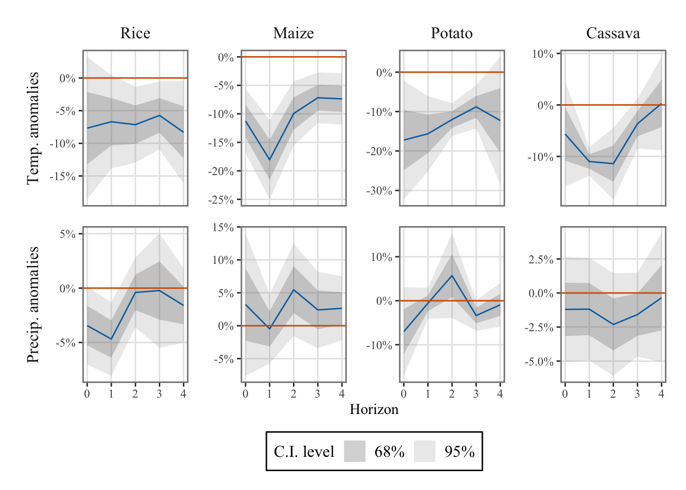
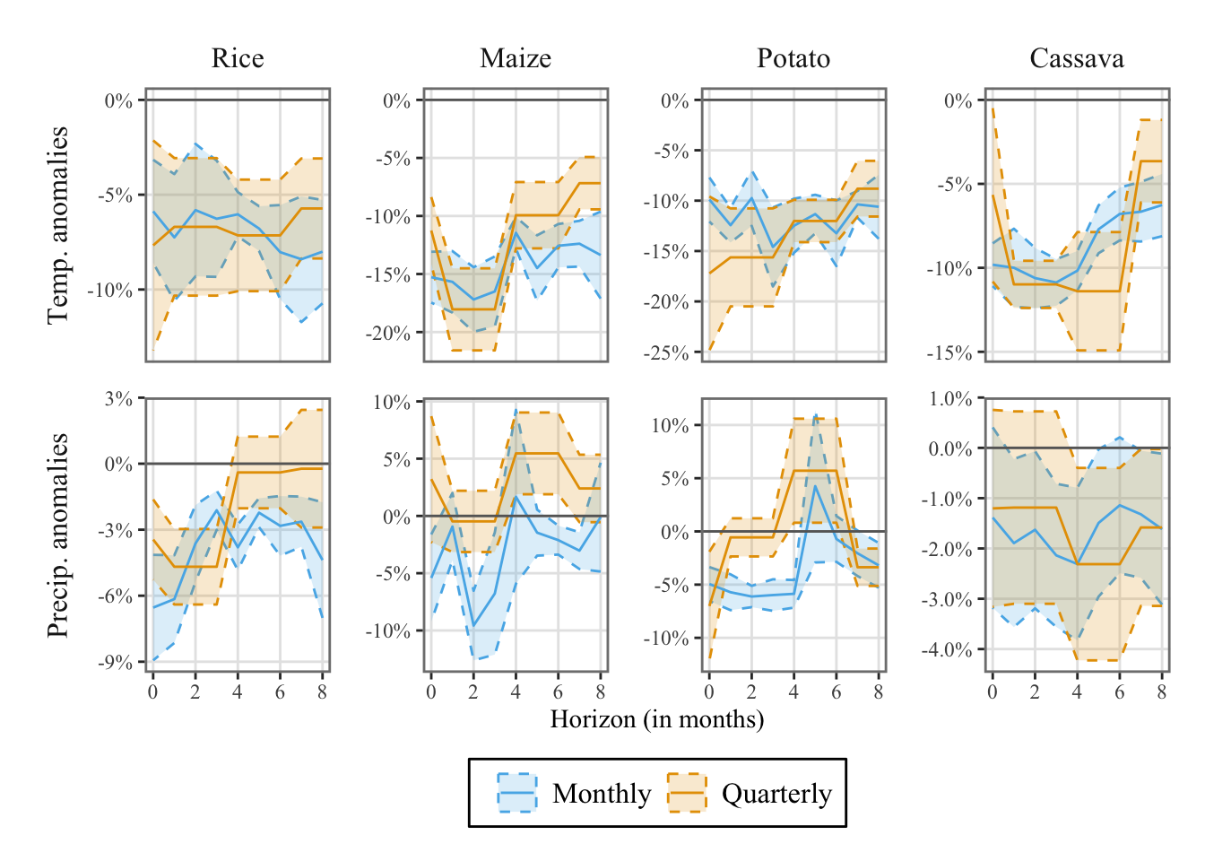
We can visualize the Impulse Response Functions (IRFs) by plotting the estimated coefficients associated with the weather variables. These coefficients represent the impact of weather on agricultural production and can provide valuable insights into the dynamics of the system. By plotting the IRFs, we can gain a better understanding of the relationship between weather variables and the response of agricultural production over time.

The data for the graphs:

df_irfs_lp_quarter <- map(resul_lp_quarter, "coefs") |> 
  list_rbind() |> 
  filter(name %in% weather_variables) |> 
  mutate(
    shock_1_sd = value * std_shock,
    lower_95 = (value - qnorm(0.975) * std) * std_shock,
    upper_95 = (value + qnorm(0.975) * std) * std_shock,
    lower_68 = (value - qnorm(0.84)  * std) * std_shock,
    upper_68 = (value + qnorm(0.84)  * std) * std_shock
  ) |> 
  mutate(
    crop = factor(
      crop, 
      levels = c("Rice", "Dent corn", "Potato", "Cassava"),
      labels = c("Rice", "Maize", "Potato", "Cassava"))
  ) |> 
  mutate(
    name = factor(
      name,
      levels = c(
        "temp_max_dev",
        "precip_sum_dev"
      ),
      labels = c(
        "Temp. anomalies", 
        "Precip. anomalies"
      )
    )
  )

For the confidence intervals:

df_irfs_lp_ci_quarter <- 
  df_irfs_lp_quarter |> 
  select(horizon, crop, name, matches("^(lower)|^(upper)", perl = TRUE)) |> 
  pivot_longer(
    cols = matches("^(lower)|^(upper)", perl = TRUE),
    names_pattern = "(.*)_(95|68)$",
    names_to = c(".value", "level")
  ) |> 
  mutate(level = str_c(level, "%"))

ggplot() +
  geom_ribbon(
    data = df_irfs_lp_ci_quarter |> filter(horizon <= 8),
    mapping = aes(
      x = horizon,
      ymin = lower, ymax = upper, fill = level),
    alpha = .2
  ) +
  geom_line(
    data = df_irfs_lp_quarter |> filter(horizon <= 8),
    mapping = aes(x = horizon, y = shock_1_sd),
    colour = "#0072B2") +
  geom_hline(yintercept = 0, colour = "#D55E00") +
  ggh4x::facet_grid2(
    name~crop, scales = "free_y", 
    independent = "y", switch = "y") +
  scale_y_continuous(labels = scales::percent) +
  labs(x = "Horizon", y = NULL) +
  scale_fill_manual(
    "C.I. level", 
    values = c("68%" = "gray10", "95%" = "gray60")
  ) +
  theme_paper() +
  theme(strip.placement = "outside")

Figure 12.1: Agricultural production response to a weather shock

12.2 Comparison with Monthly Data

Let us now load the estimations made in [Chapter @-sec-lp] with monthly dtaa to compare them with those obtained here with quarterly data.

load("../R/output/df_irfs_lp.rda")

Let us merge the IRfs. We need to make sure that the values for each quarter are repeated 3 times so that the horizons can be compared.

df_irfs_lp_comparison <- df_irfs_lp |> 
  mutate(data_type = "monthly") |> 
  bind_rows(
    df_irfs_lp_quarter |> 
      mutate(data_type = "quarterly") |> 
      mutate(count = 3) |> 
      uncount(count) |> 
      group_by(crop, horizon, name) |> 
      mutate(
        horizon = ifelse(
          horizon != 0, 
          yes = (horizon-1)*3 + row_number(), no = 0
        )
      )
  ) |> 
  mutate(
    data_type = factor(
      data_type,
      levels = c("monthly", "quarterly"),
      labels = c("Monthly", "Quarterly")
    )
  )

We do the same with confidence intervals:

df_irfs_lp_ci_comparison <- df_irfs_lp_ci |> 
  mutate(data_type = "monthly") |> 
  bind_rows(
    df_irfs_lp_ci_quarter |> 
      mutate(data_type = "quarterly") |> 
      mutate(count = 3) |> 
      uncount(count) |> 
      group_by(crop, horizon, name, level) |> 
      mutate(
        horizon = ifelse(
          horizon != 0, 
          yes = (horizon-1)*3 + row_number(), no = 0
        )
      )
  ) |> 
  mutate(
    data_type = factor(
      data_type,
      levels = c("monthly", "quarterly"),
      labels = c("Monthly", "Quarterly")
    )
  )

Then, we can plot the IRfs:

ggplot() +
  geom_ribbon(
    data = df_irfs_lp_ci_comparison |> filter(level == "68%", horizon <= 8),
    mapping = aes(
      x = horizon,
      ymin = lower, ymax = upper, fill = data_type, colour = data_type),
    alpha = .2, linetype = "dashed"
  ) +
  geom_line(
    data = df_irfs_lp_comparison |> filter(horizon <= 8),
    mapping = aes(x = horizon, y = shock_1_sd, colour = data_type)
    ) +
  scale_colour_manual(
    NULL, 
    values = c("Monthly" = "#56B4E9", "Quarterly" = "#E69F00")
    ) +
  geom_hline(yintercept = 0, colour = "gray40") +
  ggh4x::facet_grid2(
    name~crop, scales = "free_y", 
    independent = "y", switch = "y") +
  scale_y_continuous(labels = scales::percent) +
  scale_x_continuous(breaks = seq(0, 12, by = 2)) +
  labs(x = "Horizon (in months)", y = NULL) +
  scale_fill_manual(
    NULL,
    values = c("Monthly" = "#56B4E9", "Quarterly" = "#E69F00")
  ) +
  theme_paper() +
  theme(strip.placement = "outside")

Figure 12.2: Agricultural production response to a weather shock, using either monthly or quarterly data.

Acevedo, Sebastian, Mico Mrkaic, Natalija Novta, Evgenia Pugacheva, and Petia Topalova. 2020. “The Effects of Weather Shocks on Economic Activity: What Are the Channels of Impact?” Journal of Macroeconomics 65: 103207.

Jordà, Òscar. 2005. “Estimation and Inference of Impulse Responses by Local Projections.” American Economic Review 95 (1): 161–82. https://doi.org/10.1257/0002828053828518.