6  Descriptive Statistics

This chapter presents some descriptive statistics.

library(tidyverse)

── Attaching core tidyverse packages ──────────────────────── tidyverse 2.0.0 ──
✔ dplyr     1.1.4     ✔ readr     2.1.4
✔ forcats   1.0.0     ✔ stringr   1.5.0
✔ ggplot2   3.4.4     ✔ tibble    3.2.1
✔ lubridate 1.9.3     ✔ tidyr     1.3.0
✔ purrr     1.0.2     
── Conflicts ────────────────────────────────────────── tidyverse_conflicts() ──
✖ dplyr::filter() masks stats::filter()
✖ dplyr::lag()    masks stats::lag()
ℹ Use the conflicted package (<http://conflicted.r-lib.org/>) to force all conflicts to become errors

The different ggplot2 themes can be loaded:

source("../weatherperu/R/utils.R")

Let us load the data used in the local projections estimations.

load("../data/output/df_lp.rda")

We also load the weather data:

load("../data/output/weather/weather_regions_df.rda")

The map of Peru can be loaded (See (Section peru-map?) for more details on the map).

map_peru <- "../data/raw/shapefile_peru/departamentos/" |> 
  sf::st_read(quiet = TRUE)
map_peru <-
  rmapshaper::ms_simplify(input = as(map_peru, 'Spatial')) |>
  sf::st_as_sf()

6.1 Dictionary of the Variables

Table 6.1: Variables in the df dataset stored in "../data/output/df_lp.rda" file

Variable name	Type	Description
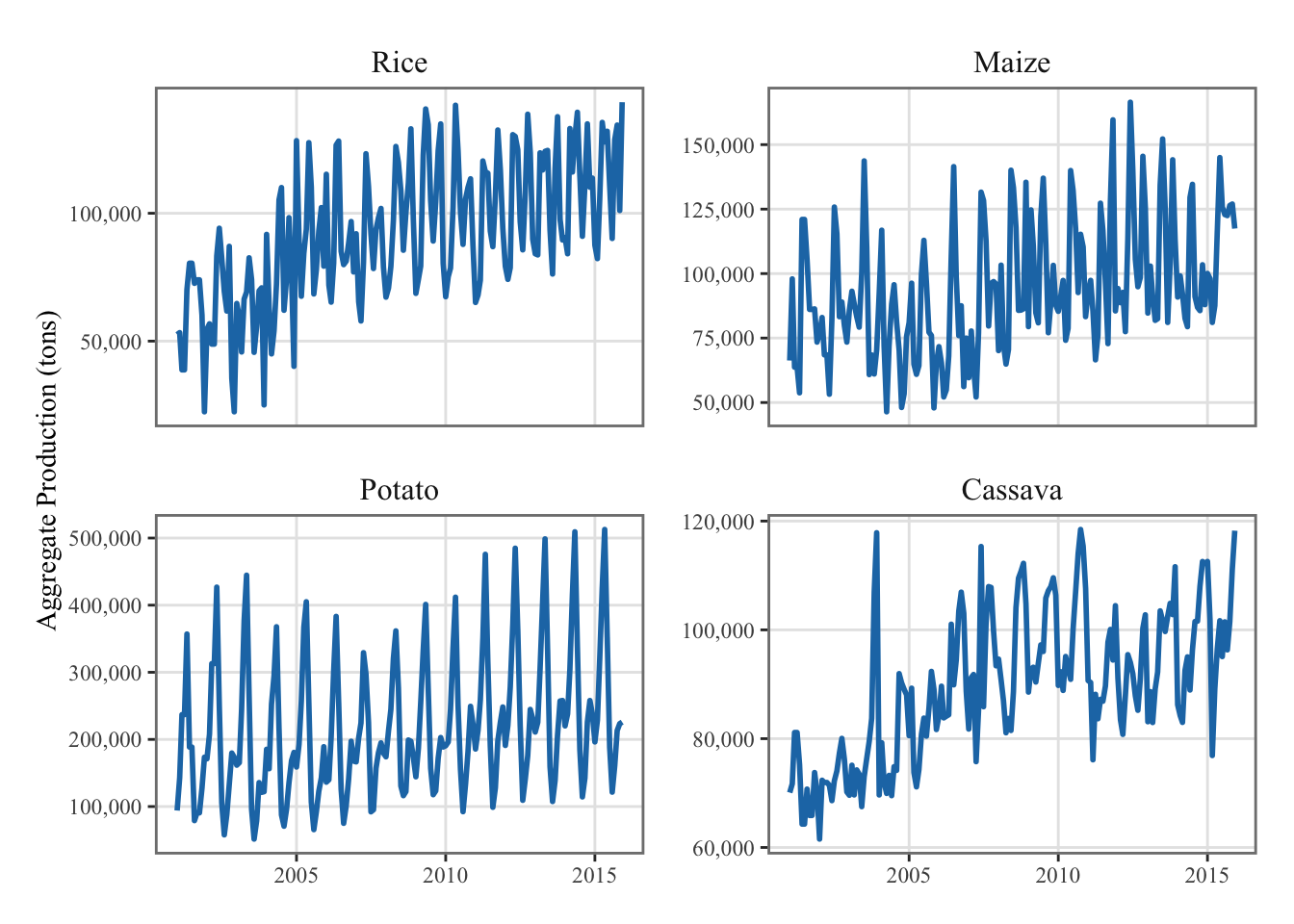
y_new	Monthly Agricultural Production (tons)
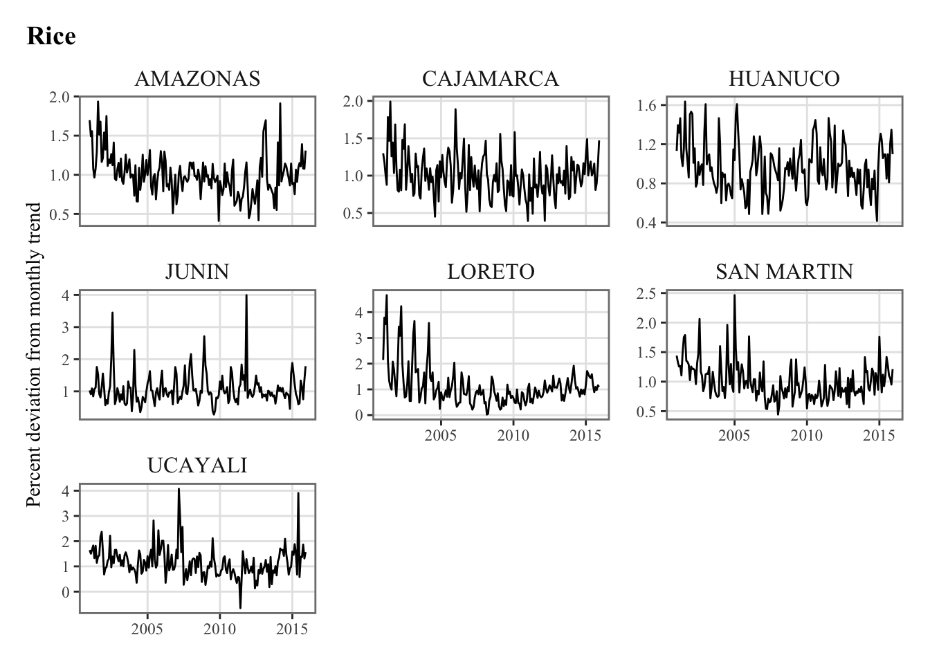
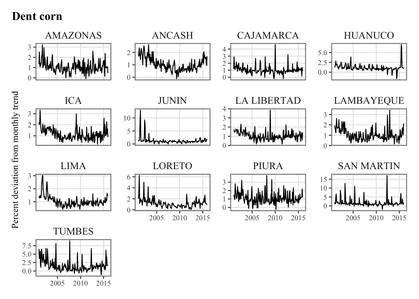
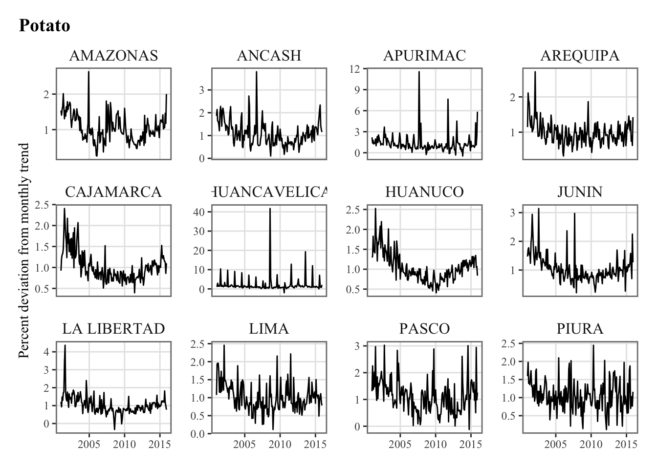
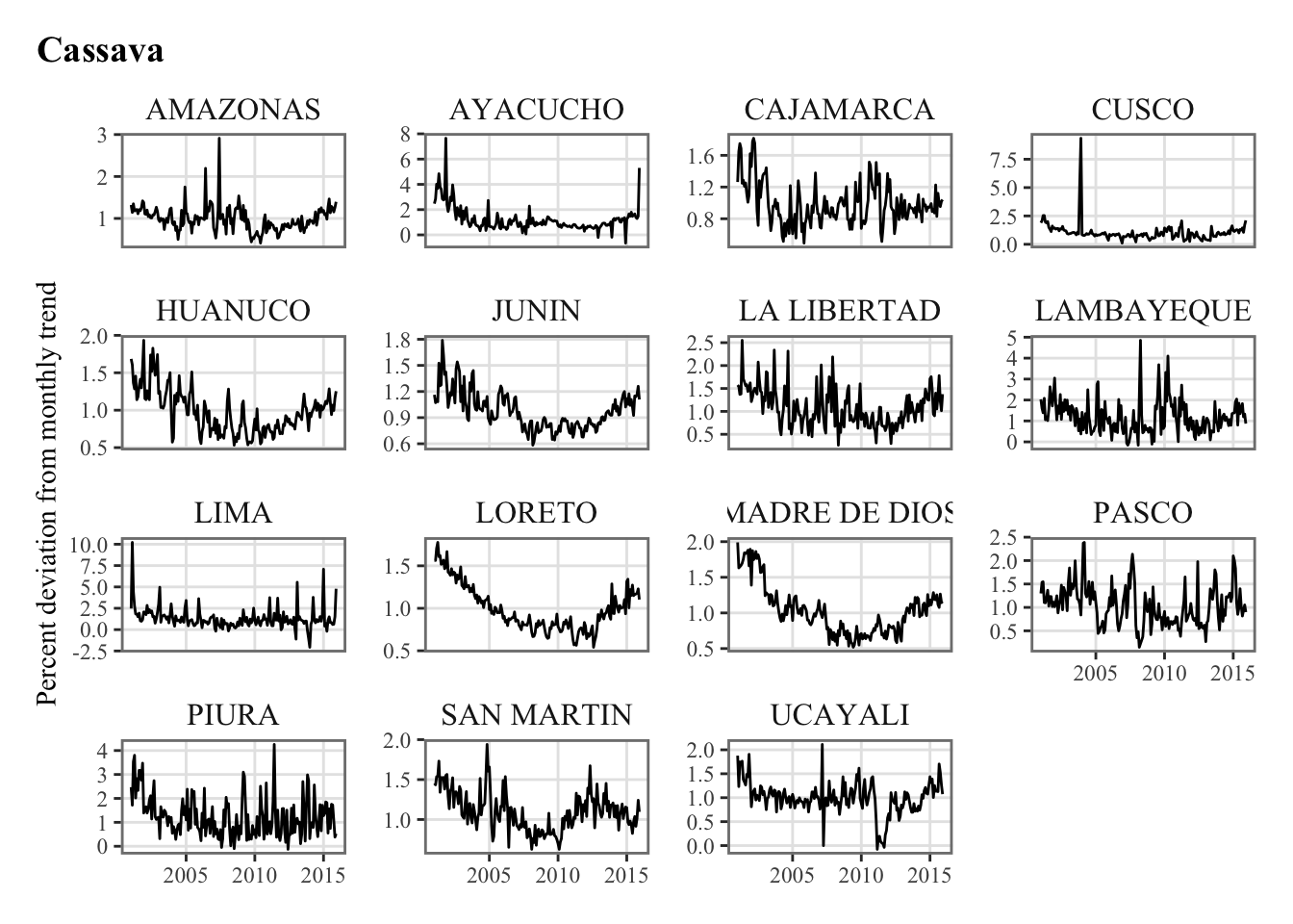
y	Monthly Agricultural Production (pct. deviation from monthly trend)
product	character	Name of the crop (in Spanish)
product_eng	character	Name of the Product (in English)
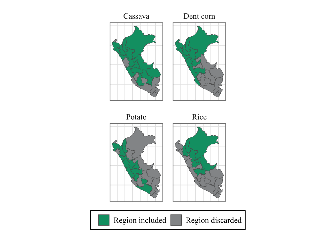
region_id	integer	Region numerical ID
region	character	Name of the region
year	numeric	Year (YYYY)
month	numeric	Month (MM)
date	Date	Date (YYYY-MM-DD)
ln_prices	numeric	Product price (log)
ln_produc	numeric	Production (log of tons)
Value_prod	numeric	Production (tons)
surf_m	numeric	Planted Surface during the current month (hectares)
Value_surfR	numeric	Harvested Surface (hectares)
Value_prices	numeric	Unit Price (Pesos)
campaign	numeric	ID of the planting campaing (starting in August)
campaign_plain	character	Years of the planting campaing (starting in August)
month_campaign	numeric	Month of the planting campaing (August = 1)
surf_lag_calend	numeric	Planted Surface laggued by the growth duration computed from the caledars (hectares)
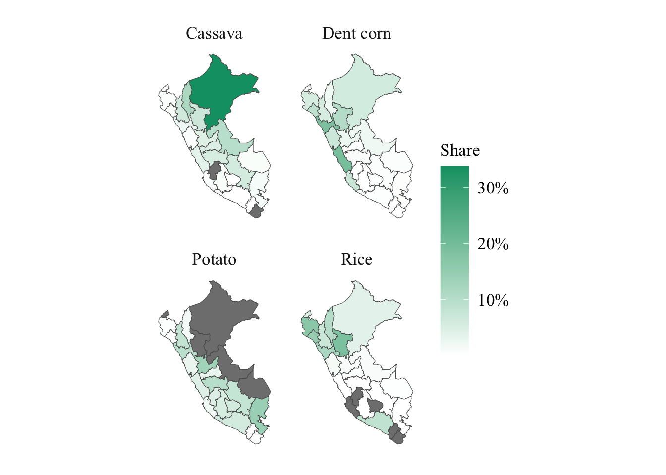
perc_product	numeric	Share of the annual production harvested at month m
perc_product_mean	numeric	Average share of the annual production harvested at month m
diff_plant_harv	numeric	Difference between planted and harvested surfaces during month m
exposition	numeric	Cumulative difference between planted and harvested surfaces
exposition_trend	numeric	Trend of the exposition using HP filter
exposition_detrended	numeric	Difference between the exposition and its trend
exposition_norm	numeric	Normalisation of the detrended exposition
temp_min	numeric	Monthly average of daily min temperature
temp_max	numeric	Monthly average of daily max temperature
temp_mean	numeric	Monthly average of daily mean temperature
precip_sum	numeric	Monthly sum of daily rainfall
perc_gamma_precip	numeric	Percentile of the monthly precipitation (Estimated Gamma Distribution)
temp_min_dev	numeric	Deviation of monthly min temperatures (temp_min) from climate normals (1986 – 2015)
temp_max_dev	numeric	Deviation of monthly max temperatures (temp_max) from climate normals (1986 – 2015)
temp_mean_dev	numeric	Deviation of monthly mean temperatures (temp_mean) from climate normals (1986 – 2015)
precip_sum_dev	numeric	Deviation of monthly total rainfall (precip_sum) from climate normals (1986 – 2015)
spi_1	numeric	SPI Drought Index, Scale = 1
spi_3	numeric	SPI Drought Index, Scale = 3
spi_6	numeric	SPI Drought Index, Scale = 6
spi_12	numeric	SPI Drought Index, Scale = 12
spei_1	numeric	SPEI Drought Index, Scale = 1
spei_3	numeric	SPEI Drought Index, Scale = 3
spei_6	numeric	SPEI Drought Index, Scale = 6
spei_12	numeric	SPEI Drought Index, Scale = 12
ONI	numeric	Oceanic Niño Index
elnino	numeric	1 if El-Niño event, 0 otherwise
lanina	numeric	1 if La-Niña event, 0 otherwise
State	numeric	State: "La Niña", "Normal", or "El Niño"
enso_start	numeric	1 if current date corresponds to the begining of one of the three states, 0 otherwise
enso_end	numeric	1 if current date corresponds to the end of one of the three states, 0 otherwise
temp_min_dev_ENSO	numeric	Deviation of Min. Temperature from ENSO Normals
temp_max_dev_ENSO	numeric	Deviation of Max. Temperature from ENSO Normals
temp_mean_dev_ENSO	numeric	Deviation of Mean Temperature from ENSO Normals
precip_sum_dev_ENSO	numeric	Deviation of Total Rainfall from ENSO Normals
gdp	numeric	GDP in percentage point, percentage deviation from trend, detrended and seasonally adjusted
ya	numeric	Agricultural GDP in percentage point, percentage deviation from trend, detrended and seasonally adjusted
rer_hp	numeric	Real exchange rate, detrended using HP filter
rer_dt_sa	numeric	Real exchange rate, detrended and seasonally adjusted
r	numeric	Interest rate, in percentage point, detrended
r_hp	numeric	Interest rate, in percentage point, detrended using HP filter
pi	numeric	Inflation rate, in percentage point
pia	numeric	Food inflation rate, in percentage point, seasonally adjusted
ind_prod	numeric	Manufacturing Production, in percentage point, percentage deviation from trend, detrended and seasonally adjusted
price_int	numeric	International commodity prices
price_int_inf	numeric	Growth rate of international commodity prices
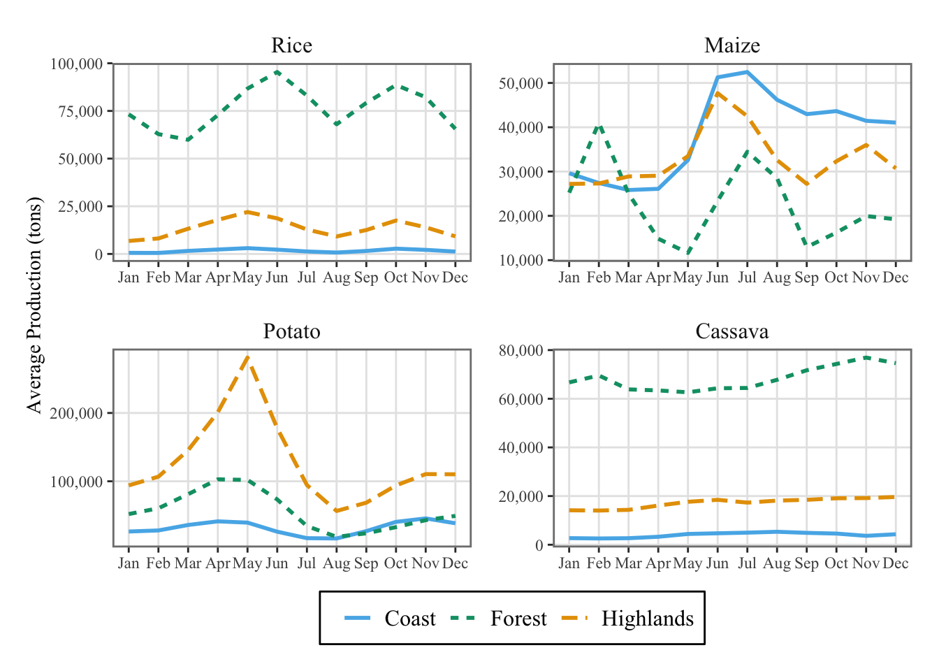
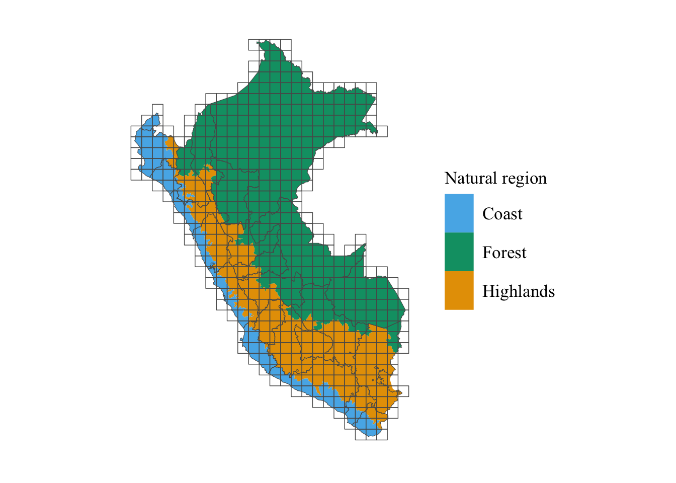
share_sierra	numeric	Share of highlands
share_selva	numeric	Share of forest
share_costa	numeric	Share of coast

6.2 Crops

We focus on the following crops:

crops <- c("Rice", "Dent corn", "Potato", "Cassava")

(tab-stats-prod?) presents some descriptive statistics about the monthly production of the selected crops, averaged over the region

df |>
  group_by(product_eng) |> 
  summarise(
    prod_mean = mean(y_new),
    prod_median = median(y_new),
    prod_sd = sd(y_new),
    prod_min = min(y_new),
    prod_max = max(y_new),
    nb_regions = length(unique(region)),
    nb_obs = n()
  ) |> 
  kableExtra::kable()

Monthly agricultural production (in Tons), per region

product_eng	prod_mean	prod_median	prod_sd	prod_min	prod_max	nb_regions	nb_obs
Cassava	5971.928	3897.6	7697.762	0	57135.0	15	2700
Dent corn	7230.704	4401.0	8496.076	0	74623.7	13	2340
Potato	18035.088	10565.0	20118.050	0	127004.9	12	2160
Rice	13090.539	4711.0	15999.357	0	100205.0	7	1260

6.2.1 National Production

Figure 6.1 provides a visual representation of the national production of each time of crop over our time sample, which is the sum of the monthly regional production.

ggplot(
  data = df |> 
    group_by(product_eng, date) |> 
    summarise(
      nat_prod = sum(y_new),
      .groups = "drop"
    ) |> 
    mutate(
      product_eng = factor(
        product_eng, 
        levels = c("Rice", "Dent corn", "Potato", "Cassava"),
        labels = c("Rice", "Maize", "Potato", "Cassava"),
      )
    )
) +
  geom_line(
    mapping = aes(x = date, y = nat_prod),
    colour = "#1f78b4",
    linewidth = 1
  ) +
  facet_wrap(~product_eng, scales = "free_y", ncol = 2) +
  labs(x = NULL, y=  "Aggregate Production (tons)") +
  scale_y_continuous(labels = scales::number_format(big.mark = ",")) +
  theme_paper()

Figure 6.1: National monthly crop production for selected cultures (in tons)

6.2.2 National production by month and type of region

In Figure 6.2, we document the regional differences and the seasonality by averaging the monthly production over the different types of natural regions.

ggplot(
  data = df |> 
    group_by(product_eng, year, month) |> 
    # Average each month at the national level
    summarise(
      prod_nat_costa = sum(y_new * share_costa),
      prod_nat_selva = sum(y_new * share_selva),
      prod_nat_sierra = sum(y_new * share_sierra),
      .groups = "drop"
    ) |> 
    pivot_longer(
      cols = c(prod_nat_costa, prod_nat_selva, prod_nat_sierra),
      names_to = "geo",
      values_to = "monthly_prod_geo"
    ) |> 
    # Average in each region type for each calendar month
    group_by(product_eng, month, geo) |> 
    summarise(
      monthly_prod_geo = mean(monthly_prod_geo),
      .groups = "drop"
    ) |> 
    mutate(
      product_eng = factor(
        product_eng, 
        levels = c("Rice", "Dent corn", "Potato", "Cassava"),
        labels = c("Rice", "Maize", "Potato", "Cassava"),
      ),
      geo = factor(
        geo,
        levels = c("prod_nat_costa", "prod_nat_selva", "prod_nat_sierra"),
        labels = c("Coast", "Forest", "Highlands")
      )
    ),
  mapping = aes(
    x = month, y = monthly_prod_geo, 
    colour = geo, linetype = geo
  )
) +
  geom_line(
    linewidth = 1
  ) +
  facet_wrap(~product_eng, scales = "free") +
  labs(x = NULL, y = "Average Production (tons)") +
  scale_colour_manual(
    NULL,
    values = c(
      "Coast" = "#56B4E9", "Forest" = "#009E73", "Highlands" = "#E69F00"
    )
  ) +
  scale_linetype_discrete(NULL) +
  scale_x_continuous(breaks= 1:12, labels = month.abb) +
  scale_y_continuous(labels = scales::number_format(big.mark = ",")) +
  theme_paper()

Figure 6.2: Crop production by months and natural regions (in tons)

6.2.3 Share of agricultural land

Let us load the share of agricultural area in the cell, for each cell of the grid (see Section 1.2 for more details on that specific grid):

load("../data/output/land/map_peru_grid_agri.rda")

Figure 6.3 presents the production distribution for each type of crop.

ggplot() +
  geom_sf(
    data = map_peru_grid_agri |> 
      mutate(share_cropland = percent_cropland / 100), 
    mapping = aes(fill = share_cropland),
    colour = "grey"
  ) +
  geom_sf(data = map_peru, fill = NA) +
  scale_fill_gradient2(
    "Share of\nagricultural\nland", 
    low = "white", high = "#61C250",
    labels = scales::label_percent()
  ) +
  theme_map_paper()

Figure 6.3: Regional distribution of crop production by administrative regions

6.2.4 Regions Used in the Local Projection Analysis

We need to know, for each region of the map, whether it is included or not in the analysis.

The number of regions used in the analysis for each crop:

df |> 
  group_by(product_eng) |> 
  summarise(nb_regions = length(unique(region_id)))

# A tibble: 4 × 2
  product_eng nb_regions
  <chr>            <int>
1 Cassava             15
2 Dent corn           13
3 Potato              12
4 Rice                 7

We can also look at the spatial distribution of these regions.

df_plot_map_regions <- 
  map_peru |> 
  left_join(
    df |> 
      select(product_eng, region) |> unique() |> 
      mutate(used = TRUE) |> 
      pivot_wider(names_from = product_eng, values_from = used),
    by = c("DEPARTAMEN" = "region")
  )

Figure 6.4 shows for each region, whether it is included (green) or not (grey).

ggplot(
  data = df_plot_map_regions |> 
    pivot_longer(cols = !!crops, values_to = "included") |> 
    mutate(
      included = replace_na(included, FALSE),
      included = factor(
        included, levels = c(TRUE, FALSE),
        labels = c("Yes", "No")
      )
    )
) +
  geom_sf(mapping = aes(fill = included)) +
  facet_wrap(~name) +
  theme_paper() +
  scale_fill_manual(
    NULL,
    values = c("Yes" = "#009E73", "No" = "#949698"),
    labels = c("Yes" = "Region included", "No" = "Region discarded")) +
  theme(
    axis.title = element_blank(),
    axis.text = element_blank(),
    axis.ticks = element_blank(),
    axis.line = element_blank()
  )

Figure 6.4: Geographic Distribution of Departments Included in the Analysis

Let us compare the previous map with the annual production. Some regions are discarded because the production is 0 for consecutive months (see Chapter 5).

Let us load the dataset obtained at the end of Chapter 5.

load("../data/output/dataset_2001_2015.rda")

We compute the crop-specific share that each region represents in the annual production.

prod_reg <- 
  data_total |> 
  group_by(region, product_eng) |> 
  summarise(
    total_production = sum(Value_prod, na.rm = T),
    .groups = "drop"
  ) |> 
  unique() |> 
  group_by(product_eng) |> 
  mutate(total_culture = sum(total_production)) |> 
  ungroup() |> 
  mutate(share = total_production / total_culture)
prod_reg

# A tibble: 122 × 5
   region   product_eng     total_production total_culture   share
   <chr>    <chr>                      <dbl>         <dbl>   <dbl>
 1 AMAZONAS Amylaceous corn           99029.      3977184. 0.0249 
 2 AMAZONAS Cassava                 1877789.     16369048. 0.115  
 3 AMAZONAS Dent corn                328864.     17750131. 0.0185 
 4 AMAZONAS Potato                   920812.     55749200. 0.0165 
 5 AMAZONAS Rice                    3998828.     38759905. 0.103  
 6 AMAZONAS Wheat                     13649.      3040741. 0.00449
 7 ANCASH   Amylaceous corn          183753.      3977184. 0.0462 
 8 ANCASH   Cassava                   99930.     16369048. 0.00610
 9 ANCASH   Dent corn               1259950.     17750131. 0.0710 
10 ANCASH   Potato                  1581346.     55749200. 0.0284 
# ℹ 112 more rows

We prepare a map dataset for each crop:

map_production_regions <- NULL
for (i in 1:length(crops)) {
  culture <- as.character(crops[i])
  map_peru_tmp <- map_peru |> 
    left_join(
      prod_reg |> 
        filter(product_eng == !!culture), 
      by = c("DEPARTAMEN" = "region")
    ) |> 
    mutate(product_eng = !!culture)
  map_production_regions <- bind_rows(map_production_regions, map_peru_tmp)
}

Figure 6.5 shows the production distribution for each type of crop.

ggplot(
  data = map_production_regions
) +
  geom_sf(
    mapping = aes(fill = share, group = DEPARTAMEN)
  ) +
  scale_fill_gradient2(
    "Share", low = "#FFC107", mid = "white", high = "#009E73",
    labels = scales::percent_format()
  ) +
  facet_wrap(~product_eng) +
  theme_map_paper()

Figure 6.5: Regional distribution of crop production by administrative regions

Now, we are interested in combining the information from Figure 6.4 and Figure 6.5, to assess the importance of the discarded series in relation to national production.

included_regions <- 
  df_plot_map_regions |> 
  pivot_longer(cols = !!crops, values_to = "included") |> 
  as_tibble() |> 
  select(IDDPTO, name, included) |> 
  mutate(included = replace_na(included, FALSE)) |> 
  rename(product_eng = name)

Figure 6.6 allows to visualize the relative importance of the discarded series in relation to the overall national agricultural production.

ggplot(
  data = map_production_regions |> 
    left_join(included_regions, by = c("IDDPTO", "product_eng")) |> 
    mutate(
      included = factor(
        included, 
        levels = c(TRUE, FALSE), 
        labels = c("Yes", "No")
      )
    )
) +
  geom_sf(
    mapping = aes(
      fill = share, group = DEPARTAMEN, 
      colour = included, linewidth = included)
  ) +
  scale_fill_gradient2(
    "Share", low = "#FFC107", mid = "white", high = "#009E73",
    labels = scales::percent_format()
  ) +
  facet_wrap(~product_eng) + 
  scale_colour_manual(
    "Included?", 
    values = c("Yes" = "#56B4E9", "No" = "gray")
  ) +
  scale_linewidth_manual(
    "Included?", 
    values = c("Yes" = .6, "No" = .2)
  ) +
  theme_map_paper()

Figure 6.6: Comparison of Discarded Series with National Production

6.3 Natural regions

Let us now focus on the natural regions: Coast, Forest, Highlands.

First, we load the map (see Section 4.1):

map_regiones_naturales <-  sf::st_read(
  str_c(
    "../data/raw/shapefile_peru/regiones_naturales/",
    "region natural_geogpsperu_JuanPabloSuyoPomalia.geojson"
  ),
  quiet = TRUE
)

Let us prepare a map:

map_regiones_naturales <-
  rmapshaper::ms_simplify(input = as(map_regiones_naturales, 'Spatial')) |> 
  sf::st_as_sf() |> 
  mutate(
    Natural_region = case_when(
      Nm_RegNat == "Costa" ~ "Coast",
      Nm_RegNat == "Selva" ~ "Forest",
      Nm_RegNat == "Sierra" ~ "Highlands"
    )
  )

We use the following colours for each type of region:

cols <- c("Coast" = "#56B4E9", "Forest" = "#009E73", "Highlands" = "#E69F00")

Figure 6.7 shows these regions, and adds the grid used with the weather data from Chapter 1 as well as the regional boundaries used in the analysis.

ggplot(data = map_regiones_naturales) +
  geom_sf(mapping = aes(fill = Natural_region), lwd = 0) +
  scale_fill_manual(values = cols, name = "Natural region") +
  geom_sf(data = map_peru, fill = NA) +
  geom_sf(data = map_peru_grid_agri, fill = NA, lwd = 0.25) +
  theme_map_paper()

Figure 6.7: Natural Regions in Peru

6.4 Correlations Between Agricultural Production and the Weather

Let us compute the correlation between the agricultural production and our various weather variables. Recall from Chapter 5 that the agricultural production is defined as the percent deviation from the monthly trend.

The name of the weather variables:

name_weather_variables <- 
  weather_regions_df |> 
  select(where(is.numeric)) |> 
  select(-year, -month) |> 
  colnames()
name_weather_variables

 [1] "temp_min"          "temp_max"          "temp_mean"        
 [4] "precip_sum"        "perc_gamma_precip" "temp_min_dev"     
 [7] "temp_max_dev"      "temp_mean_dev"     "precip_sum_dev"   
[10] "spi_1"             "spi_3"             "spi_6"            
[13] "spi_12"            "spei_1"            "spei_3"           
[16] "spei_6"            "spei_12"          

df |>
  select(product_eng, y, !!!syms(name_weather_variables)) |>
  na.omit() |>
  nest(.by = product_eng) |> 
  mutate(
    correlation = map(
      data, ~cor(.x) |> 
        data.frame() |> 
        as_tibble(rownames = "var")
    )
  ) |> 
  select(-data) |> 
  unnest(correlation) |> 
  select(Crop = product_eng, Variable = var, y) |> 
  pivot_wider(names_from = Crop, values_from = y) |> 
  mutate(across(where(is.numeric), ~round(.x, 2))) |> 
  knitr::kable()

Table 6.2: Correlations between the weather and the agricultural production

Variable	Cassava	Dent corn	Potato	Rice
y	1.00	1.00	1.00	1.00
temp_min	0.01	0.05	-0.10	0.09
temp_max	-0.01	0.05	-0.06	0.08
temp_mean	0.00	0.05	-0.09	0.09
precip_sum	-0.05	-0.02	-0.03	0.07
perc_gamma_precip	-0.01	-0.04	-0.01	-0.10
temp_min_dev	0.00	0.01	0.02	-0.01
temp_max_dev	-0.08	-0.07	-0.01	-0.04
temp_mean_dev	-0.06	-0.04	0.00	-0.03
precip_sum_dev	0.00	-0.03	-0.01	-0.11
spi_1	-0.01	-0.04	-0.01	-0.09
spi_3	0.00	-0.05	-0.02	-0.11
spi_6	-0.01	-0.05	0.01	-0.12
spi_12	-0.01	-0.03	0.02	-0.12
spei_1	-0.01	-0.04	-0.01	-0.09
spei_3	0.00	-0.04	-0.02	-0.12
spei_6	0.00	-0.04	0.01	-0.12
spei_12	0.00	-0.02	0.02	-0.12

6.5 Summary Statistics for the Local Projection Data

The number of observation in each region and crops (ordered by decreasing values):

df |> 
  count(product_eng, region_id) |> 
  arrange(n)

# A tibble: 47 × 3
   product_eng region_id     n
   <chr>       <fct>     <int>
 1 Cassava     1           180
 2 Cassava     5           180
 3 Cassava     6           180
 4 Cassava     7           180
 5 Cassava     9           180
 6 Cassava     11          180
 7 Cassava     12          180
 8 Cassava     13          180
 9 Cassava     14          180
10 Cassava     15          180
# ℹ 37 more rows

Let us plot the agricultural production series for each crop in each region.

plots_crops_lp <- vector(mode = "list", length = length(crops))
for (i_crop in 1:length(crops)) {
  current_crop <- crops[i_crop]
  # The series in each region for the current crop
  p_crop_lp <- 
    ggplot(
    data = df |> filter(product_eng == !!current_crop),
    mapping = aes(x = date, y = y)
  ) +
    geom_line() +
    facet_wrap(~region, scales = "free_y") +
    labs(
      title = current_crop, x = NULL,
      y = "Percent deviation from monthly trend") +
    theme_paper()
  plots_crops_lp[[i_crop]] <- p_crop_lp
}
names(plots_crops_lp) <- crops

Rice

print(plots_crops_lp[["Rice"]])

Figure 6.8: Regional Production of Rice (Deviation from Monthly Trend)

Maize (Dent corn)

print(plots_crops_lp[["Dent corn"]])

Figure 6.9: Regional Production of Maize (Deviation from Monthly Trend)

Potato

print(plots_crops_lp[["Potato"]])

Figure 6.10: Regional Production of Potato (Deviation from Monthly Trend)

Cassava

print(plots_crops_lp[["Cassava"]])

Figure 6.11: Regional Production of Cassava (Deviation from Monthly Trend)

library(gtsummary)
df |>
  tbl_summary(
    include = c(
      "product_eng",
      # Production
      "y_new", "y",
      # Weather
      "temp_max_dev", "perc_gamma_precip",
      # Control
      "rer", "r", "pi", "ind_prod",
      # Type of region
      "share_costa", "share_selva", "share_sierra"
    ),
    by = product_eng,
    type = all_continuous() ~ "continuous2",
    statistic = list(
      all_continuous() ~ c("{mean} ({sd})", "{median} ({p25}, {p75})"),
      all_categorical() ~ "{n} ({p}%)"),
    digits = list(
      all_continuous() ~ 2,
      all_categorical() ~ 0
    )
  ) |> 
  add_overall(col_label = "Whole sample") |> 
  modify_header(label ~ "**Variable**") |> 
  modify_spanning_header(
    c("stat_1", "stat_2", "stat_3", "stat_4") ~ "**Crop**"
  ) |> 
  add_stat_label(
    label = list(
      all_continuous() ~ c("Mean (SD)", "Median (IQR)"),
      all_categorical() ~ "n (%)"
    )
  )

Table 6.3:

Descriptive Statistics of the Data Used in the Local Projections

Variable	Overall, N = 8,460	Crop
		Cassava, N = 2,700	Dent corn, N = 2,340	Potato, N = 2,160	Rice, N = 1,260
Monthly Agricultural Production (tons)
Mean (SD)	10,460.27 (14,327.01)	5,971.93 (7,697.76)	7,230.70 (8,496.08)	18,035.09 (20,118.05)	13,090.54 (15,999.36)
Median (IQR)	4,882.99 (1,455.01, 12,918.38)	3,897.60 (1,025.93, 6,886.48)	4,401.00 (1,142.75, 10,385.17)	10,565.00 (2,950.50, 26,581.24)	4,711.00 (1,300.09, 21,315.01)
Monthly Agricultural Production (pct. deviation from monthly trend)
Mean (SD)	1.12 (0.92)	1.08 (0.62)	1.18 (1.03)	1.14 (1.26)	1.05 (0.46)
Median (IQR)	0.98 (0.76, 1.27)	0.98 (0.78, 1.24)	0.99 (0.72, 1.37)	0.99 (0.76, 1.29)	0.97 (0.79, 1.20)
Deviation of Max. Temperature from Normals
Mean (SD)	0.06 (0.58)	0.07 (0.59)	0.04 (0.59)	0.10 (0.59)	0.02 (0.55)
Median (IQR)	0.03 (-0.32, 0.43)	0.04 (-0.32, 0.44)	0.01 (-0.33, 0.39)	0.06 (-0.29, 0.49)	-0.01 (-0.34, 0.38)
Precipitation Shock (Percentile from Gamma Dist.)
Mean (SD)	0.51 (0.25)	0.51 (0.25)	0.49 (0.26)	0.51 (0.26)	0.53 (0.24)
Median (IQR)	0.52 (0.30, 0.72)	0.53 (0.30, 0.73)	0.49 (0.27, 0.71)	0.52 (0.29, 0.73)	0.55 (0.33, 0.73)
rer
Mean (SD)	1.00 (0.04)	1.00 (0.04)	1.00 (0.04)	1.00 (0.04)	1.00 (0.04)
Median (IQR)	1.00 (0.97, 1.02)	1.00 (0.97, 1.02)	1.00 (0.97, 1.02)	1.00 (0.97, 1.02)	1.00 (0.97, 1.02)
Interest rate (pp)
Mean (SD)	4.06 (1.96)	4.06 (1.96)	4.06 (1.96)	4.06 (1.96)	4.06 (1.96)
Median (IQR)	3.94 (2.99, 4.48)	3.94 (2.99, 4.48)	3.94 (2.99, 4.48)	3.94 (2.99, 4.48)	3.94 (2.99, 4.48)
Inflation rate (pp)
Mean (SD)	0.22 (0.26)	0.22 (0.26)	0.22 (0.26)	0.22 (0.26)	0.22 (0.26)
Median (IQR)	0.24 (0.03, 0.38)	0.24 (0.03, 0.38)	0.24 (0.03, 0.38)	0.24 (0.03, 0.38)	0.24 (0.03, 0.38)
Manufacturing Prod. (pp)
Mean (SD)	-0.16 (5.78)	-0.16 (5.78)	-0.16 (5.78)	-0.16 (5.78)	-0.16 (5.78)
Median (IQR)	-0.30 (-3.93, 3.99)	-0.30 (-3.93, 3.99)	-0.30 (-3.93, 3.99)	-0.30 (-3.93, 3.99)	-0.30 (-3.93, 3.99)
Share of coastal areas in the region
Mean (SD)	0.22 (0.32)	0.18 (0.31)	0.38 (0.39)	0.20 (0.25)	0.02 (0.04)
Median (IQR)	0.00 (0.00, 0.42)	0.00 (0.00, 0.42)	0.29 (0.00, 0.82)	0.05 (0.00, 0.41)	0.00 (0.00, 0.00)
Share of forest areas in the region
Mean (SD)	0.42 (0.39)	0.50 (0.39)	0.33 (0.39)	0.24 (0.30)	0.74 (0.26)
Median (IQR)	0.44 (0.00, 0.83)	0.51 (0.05, 1.00)	0.05 (0.00, 0.54)	0.03 (0.00, 0.47)	0.83 (0.44, 1.00)
Share of highland areas in the region
Mean (SD)	0.36 (0.29)	0.32 (0.28)	0.29 (0.26)	0.55 (0.26)	0.24 (0.24)
Median (IQR)	0.46 (0.05, 0.56)	0.31 (0.00, 0.53)	0.18 (0.05, 0.53)	0.54 (0.42, 0.62)	0.17 (0.00, 0.52)