4  Other Data

4.1 Natural Regions

We calculate the share of each type of natural region using data from the Geo GPS Peru website: https://www.geogpsperu.com/2019/11/mapa-de-regiones-naturales-costa-sierra.html

library(tidyverse)

── Attaching core tidyverse packages ──────────────────────── tidyverse 2.0.0 ──
✔ dplyr     1.1.4     ✔ readr     2.1.4
✔ forcats   1.0.0     ✔ stringr   1.5.0
✔ ggplot2   3.4.4     ✔ tibble    3.2.1
✔ lubridate 1.9.3     ✔ tidyr     1.3.0
✔ purrr     1.0.2     
── Conflicts ────────────────────────────────────────── tidyverse_conflicts() ──
✖ dplyr::filter() masks stats::filter()
✖ dplyr::lag()    masks stats::lag()
ℹ Use the conflicted package (<http://conflicted.r-lib.org/>) to force all conflicts to become errors

library(lubridate)
library(sf)

Linking to GEOS 3.11.0, GDAL 3.5.3, PROJ 9.1.0; sf_use_s2() is TRUE

library(rmapshaper)

The legacy packages maptools, rgdal, and rgeos, underpinning the sp package,
which was just loaded, will retire in October 2023.
Please refer to R-spatial evolution reports for details, especially
https://r-spatial.org/r/2023/05/15/evolution4.html.
It may be desirable to make the sf package available;
package maintainers should consider adding sf to Suggests:.
The sp package is now running under evolution status 2
     (status 2 uses the sf package in place of rgdal)

library(raster)

Loading required package: sp

Attaching package: 'raster'

The following object is masked from 'package:dplyr':

    select

library(stars)

Loading required package: abind

library(readxl)

4.1.1 Import Data

We first import the Peruvian map:

sf::sf_use_s2(FALSE)

Spherical geometry (s2) switched off

# Map of the administrative regions 
map_peru <- sf::st_read("../data/raw/shapefile_peru/departamentos/", quiet = T)

map_peru <-
  rmapshaper::ms_simplify(input = as(map_peru, 'Spatial')) |>
  st_as_sf()

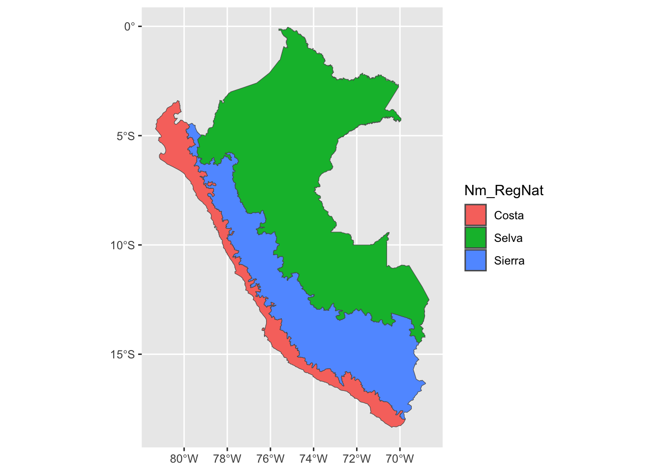
Then, we load the map with the definition of the natural regions:

# Map of the natural regions 
map_regiones_naturales <-  sf::st_read(
  str_c("../data/raw/shapefile_peru/regiones_naturales/",
        "region natural_geogpsperu_JuanPabloSuyoPomalia.geojson"
  ),
  quiet = T
)

As the file contains a lot of unecessary details, we simplify the polygons:

map_regiones_naturales <-
  rmapshaper::ms_simplify(input = as(map_regiones_naturales, 'Spatial')) |>
  st_as_sf()

Let us plot the map:

ggplot(data = map_regiones_naturales) +
  geom_sf(mapping = aes(fill = Nm_RegNat))

Figure 4.1: Map with the Natual Regions (Source: Geo GPS Peru)

4.1.2 Share of Natural Region in Each Administrative Region

We calculate the share of each type of natural region in each administrative region.

natural_region_dep <- vector(mode = "list", length = nrow(map_peru))

Looping over each administrative region:

for (i in 1:nrow(map_peru)) {
  natural_region_dep_i <- 
    st_intersection(map_peru[i,],  map_regiones_naturales) |> 
    dplyr::mutate(area_cell_intersect = st_area(geometry)) |> 
    mutate(area_cell_sqkm = units::drop_units(area_cell_intersect)*10^-6) |> 
    mutate(
      area = sum(area_cell_sqkm),
      area_pct = area_cell_sqkm/area) |> 
    dplyr::select(region = DEPARTAMEN, natural_reg = Nm_RegNat, area_pct) |> 
    as_tibble() |> 
    dplyr::select(-geometry)
  
  natural_region_dep[[i]] <- natural_region_dep_i
}

Binding the results:

natural_region_dep <- 
  dplyr::bind_rows(natural_region_dep) |> 
  dplyr::mutate(natural_reg = str_c("share_", str_to_lower(natural_reg))) |> 
  tidyr::pivot_wider(
    names_from = natural_reg, 
    values_from = area_pct, 
    values_fill = 0
  )

natural_region_dep |>
  dplyr::mutate(test = share_sierra + share_selva + share_costa)

# A tibble: 25 × 5
   region       share_sierra share_selva share_costa  test
   <chr>               <dbl>       <dbl>       <dbl> <dbl>
 1 AMAZONAS            0.169   0.831        0            1
 2 ANCASH              0.709   0            0.291        1
 3 APURIMAC            1.00    0.0000420    0            1
 4 AREQUIPA            0.595   0            0.405        1
 5 AYACUCHO            0.943   0.0568       0.000172     1
 6 CAJAMARCA           0.525   0.370        0.105        1
 7 CALLAO              0       0            1            1
 8 CUSCO               0.487   0.513        0            1
 9 HUANCAVELICA        1.00    0.0000275    0.000132     1
10 HUANUCO             0.555   0.445        0            1
# ℹ 15 more rows

We add labels to the columns:

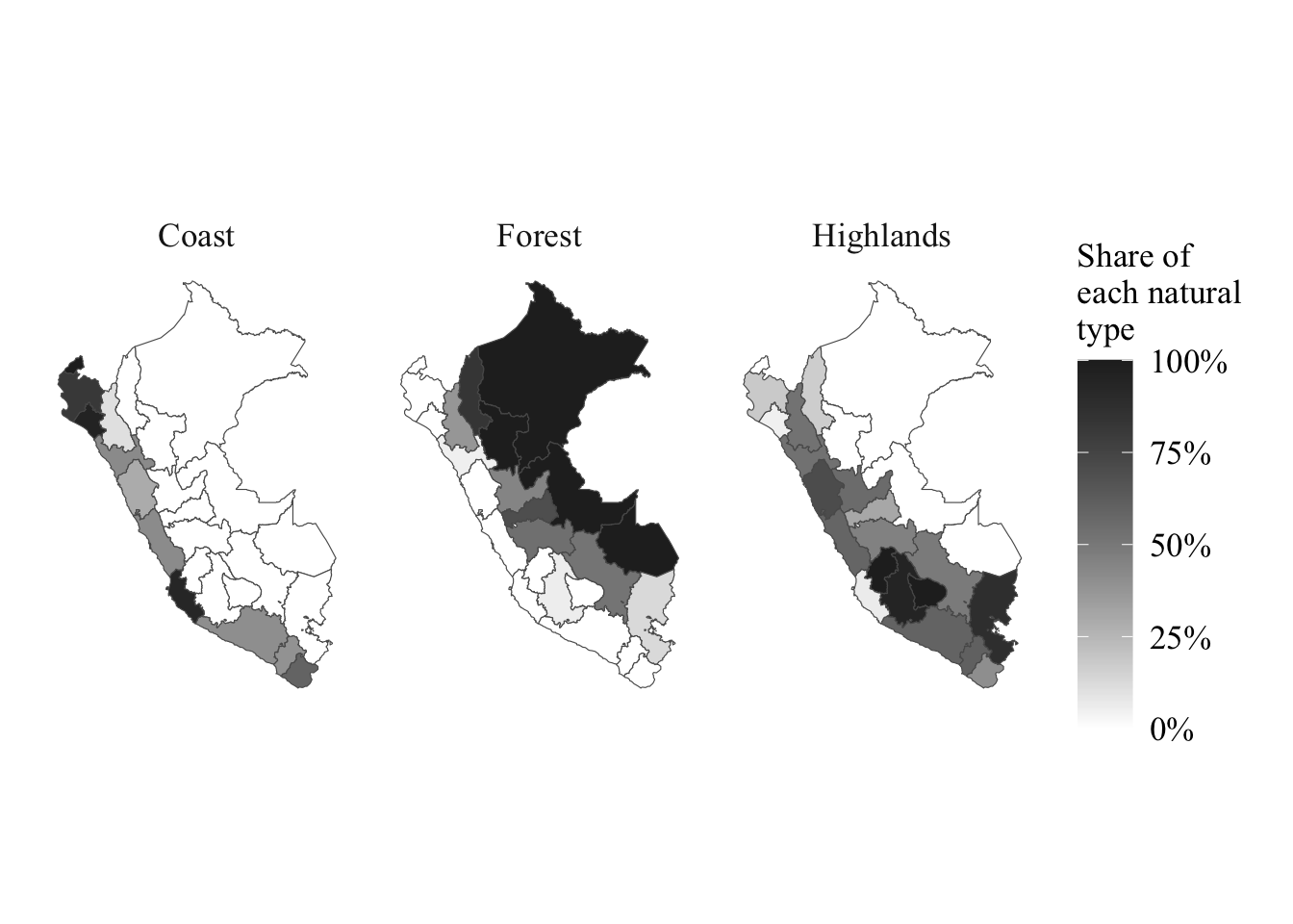
natural_region_dep <- 
  natural_region_dep |> 
  labelled::set_variable_labels(
    region = "Name of the region",
    share_costa = "Share of coastal areas in the region",
    share_selva = "Share of forest areas in the region",
    share_sierra = "Share of highland areas in the region"
  )

And the results can be saved:

save(natural_region_dep, file =  "../data/output/natural_region_dep.rda")

Let us plot the share of each type of natural regions in each administrative region on a map. We first prepare the data.

map_peru_nat_regions <- NULL
# nat_level <- "share_sierra"
for (nat_level in c("share_sierra", "share_selva", "share_costa")) {
  map_peru_nat_reg_tmp <- 
    map_peru |> 
    dplyr::left_join(
      natural_region_dep |> 
        tidyr::pivot_longer(cols = c(share_sierra, share_selva, share_costa),
                            names_to = "natural_region", values_to = "share_natural") |> 
        filter(natural_region == !!nat_level),
      by = c("DEPARTAMEN" = "region")
    )
  map_peru_nat_regions <- dplyr::bind_rows(map_peru_nat_regions, map_peru_nat_reg_tmp)
}

Then, we can create the maps.

source("../weatherperu/R/utils.R")
p <- 
  ggplot(
    data = map_peru_nat_regions |> 
      mutate(
        natural_region = factor(
          natural_region,
          levels = c("share_costa", "share_selva", "share_sierra"),
          labels = c("Coast", "Forest", "Highlands")
        )
      )
    ) +
  geom_sf(mapping = aes(fill = share_natural, group = DEPARTAMEN)) +
  scale_fill_gradient2(
    "Share of\neach natural\ntype", 
    low = "#FFC107", mid = "white", high = "gray15",
    breaks = .25*0:4,
    labels = scales::percent(.25*0:4)
  ) +
  facet_wrap(~natural_region) +
  theme_map_paper()

p

Figure 4.2: Share of each type of natural regions

4.2 Content of the dataset

Table 4.1: Variables in the natural_region_dep file

Variable name	Type	Description
region	character	Administrative Name of the Region
share_sierra	numeric	Share of highlands
share_selva	numeric	Share of forest
share_costa	numeric	Share of coast

5 El Niño–Southern Oscillation

Peru is exposed to the El Niño Southern Oscillation (ENSO) phenomenon. This phenomenon is due to irregular cyclical variations in sea surface temperatures and air pressure of the Pacific Ocean. The ENSO phenomenon is composed of two main phases: the warming phase El Niño, characterized by warmer ocean temperatures in the tropical western Pacific, and the cooling phase La Niña, with a cooling of the ocean surface.

The ENSO variations are classified using the Oceanic Niño Index, which computes a three-months average of the sea surface temperature anomalies in the central and eastern tropical Pacific Ocean. We collect this index from the Golden Gate Weather Service. An El Niño (or La Niña) event is defined by a five consecutive three-months periods with an index above 0.5 (or below -0.5 for a La Niña event).

ONI_temp <- read_excel(
  path = "../data/raw/Weather/ONI.xlsx", 
  sheet = "ONI", 
  col_types = "text") |> 
  pivot_longer(cols = -c(Year), names_to = "month") |> 
  mutate(
    elnino = ifelse(as.numeric(value) >  0.49, yes = 1, no = 0),
    lanina = ifelse(as.numeric(value) < -0.49, yes = 1, no = 0)) |> 
  filter(Year %in% c(2000: 2016)) |> 
  mutate(
    date = lubridate::ymd(str_c(Year,  "-", month, "-01")), 
    State = case_when(
      elnino == 1 ~ "El Niño", 
      lanina == 1 ~ "La Niña", 
      (elnino == 0 & lanina == 0) ~ "Normal",
      TRUE ~ "NA"
    )) |> 
  mutate(
    date_start = ifelse(State != lag(State), yes = 1, no = 0), 
    date_end   = ifelse(State != lead(State), yes = 1, no = 0)) |> 
  rename(ONI = value) |> 
  mutate(ONI = as.numeric(ONI))

ONI_temp$date_start[1] <- 1
ONI_temp$date_end[nrow(ONI_temp)] <- 1

We add labels to the columns:

ONI_temp <- 
  ONI_temp |> 
  labelled::set_variable_labels(
    Year = "Year",
    month = "Month",
    ONI = "Oceanic Niño Index",
    elnino = "Is El-Niño Event",
    lanina = "Is La-Niña Event",
    date = "Date",
    State = "ENSO State",
    date_start = "Is event start month",
    date_end = "Is event end month"
  )

Let us save this data for later use:

save(ONI_temp, file = "../data/output/weather/ONI_temp.rda")

5.1 Content of the dataset

Table 5.1: Variables in the ONI_temp file

Variable name	Type	Description
Year	character	Year (YYYY)
month	character	Month (MM)
ONI	numeric	Oceanic Niño Index
elnino	numeric	1 if El-Niño event, 0 otherwise
lanina	numeric	1 if La-Niña event, 0 otherwise
date	numeric	Date of the beginning of the month (YYYY-MM-DD)
State	numeric	State: "La Niña", "Normal", or "El Niño"
date_start	numeric	1 if current date corresponds to the begining of one of the three states, 0 otherwise
date_end	numeric	1 if current date corresponds to the end of one of the three states, 0 otherwise