4  Generalized Richards Model: estimates

This section provides the codes used to analyse the estimated values of \(P\) and \(\alpha\) (see Chapter 2)

library(tidyverse)

── Attaching core tidyverse packages ──────────────────────── tidyverse 2.0.0 ──
✔ dplyr     1.1.3     ✔ readr     2.1.4
✔ forcats   1.0.0     ✔ stringr   1.5.0
✔ ggplot2   3.4.4     ✔ tibble    3.2.1
✔ lubridate 1.9.3     ✔ tidyr     1.3.0
✔ purrr     1.0.2     
── Conflicts ────────────────────────────────────────── tidyverse_conflicts() ──
✖ dplyr::filter() masks stats::filter()
✖ dplyr::lag()    masks stats::lag()
ℹ Use the conflicted package (<http://conflicted.r-lib.org/>) to force all conflicts to become errors

Let us load the results:

load("./estim/resul_fit_countries.rda")

4.1 Exploration of the Results

The complete set of estimated parameters (using NLS) can be accessed as follows:

estimates_nls <- 
  map(resul_fit_countries, "nls") |> 
  map_df("estimates", .id = "country") |> 
  mutate(estim = "nls")
estimates_nls |> 
  DT::datatable(options = list(
    searching = TRUE,
    pageLength = 10,
    lengthMenu = c(5, 10, 15, 20)
  ))

Let us visualize these estimates on boxplots. Let us first load the list of countries and the theme used for the graphs.

load("./data/output//list_countries.rda")
library(grid)
load("./assets/theme_paper.rda")

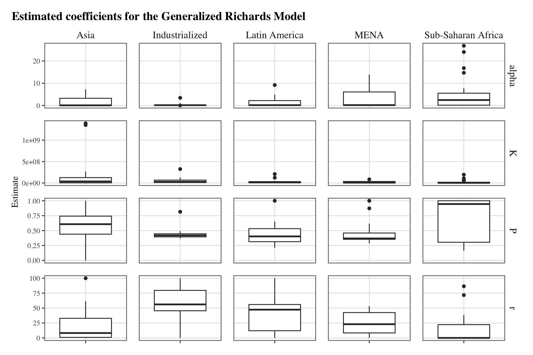
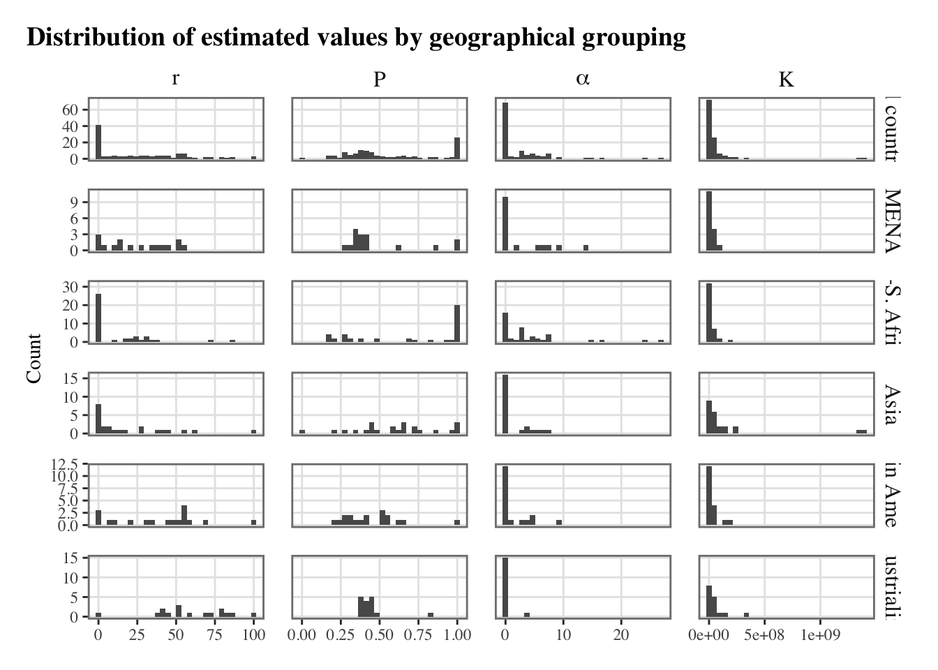
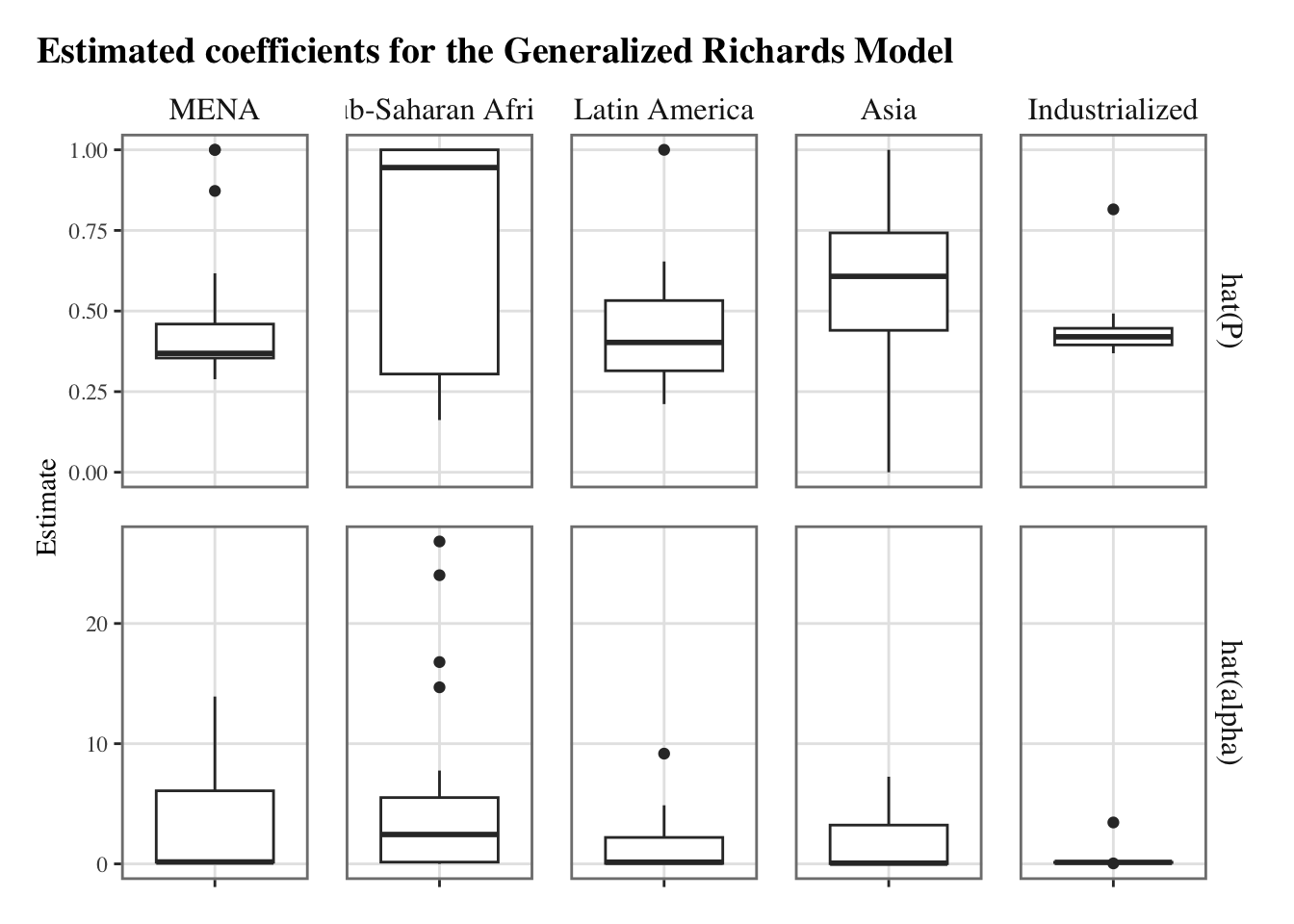
ggplot(
  data = estimates_nls |> 
    left_join(list_countries) |> 
    pivot_longer(cols = c(r, P, alpha, K)) |> 
    group_by(name, group)
) +
  geom_boxplot(
    mapping = aes(x = estim, y = value),
    na.rm = TRUE
  ) +
  facet_grid(name ~ group, scales = "free") + 
  labs(
    x = NULL, y = "Estimate",
    title = "Estimated coefficients for the Generalized Richards Model"
  ) +
  theme_paper() +
  theme(axis.text.x = element_blank())

Joining with `by = join_by(country)`

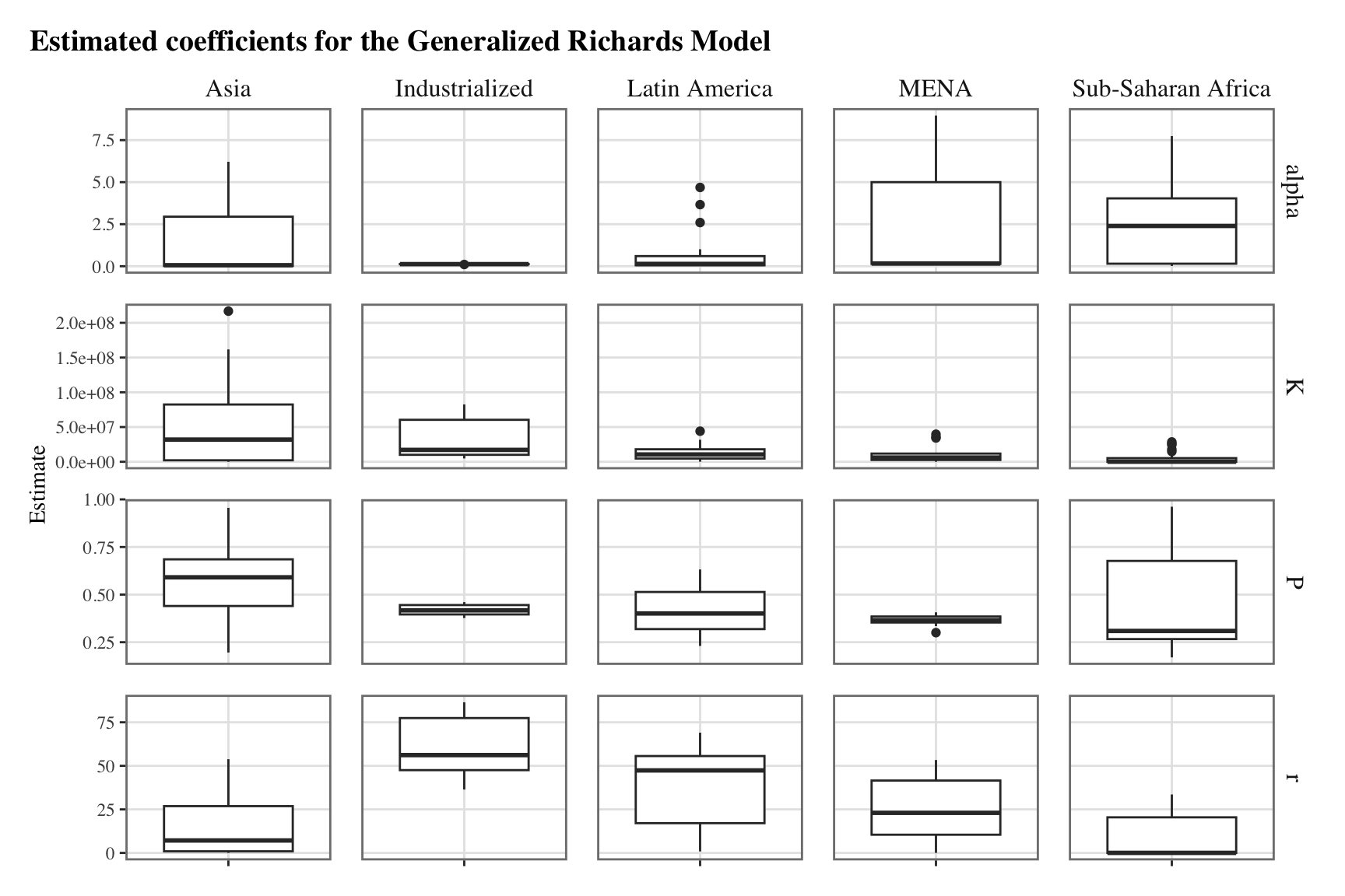
The same graph can be reproduced while removing outliers, to have a better idea of the variability between countries. We define a function to remove the outliers, as suggested by Andrew Baxter on Stack overflow:

filter_lims <- function(x) {
  l <- boxplot.stats(x)$stats[1]
  u <- boxplot.stats(x)$stats[5]
  
  for (i in 1:length(x)) {
    x[i] <- ifelse(x[i]>l & x[i]<u, x[i], NA)
  }
  return(x)
}

ggplot(
  data = estimates_nls |> 
    left_join(list_countries) |> 
    pivot_longer(cols = c(r, P, alpha, K)) |> 
    group_by(name, group) |> 
    mutate(value2 = filter_lims(value))
) +
  geom_boxplot(
    mapping = aes(x = estim, y = value2),
    na.rm = TRUE
  ) +
  facet_grid(name ~ group, scales = "free") + 
  labs(
    x = NULL, y = "Estimate",
    title = "Estimated coefficients for the Generalized Richards Model"
  ) +
  theme_paper() +
  theme(axis.text.x = element_blank())

Joining with `by = join_by(country)`

The Root Mean Squared Errors:

rmse_nls <- 
  map(resul_fit_countries, "nls") |> 
  map("rmse") |> 
  map_df(as_tibble, .id = "country") |> 
  mutate(estim = "nls")

rmse <-
  rmse_nls |> 
  pivot_wider(names_from = estim, values_from = value)

Let us put these values in a table:

rmse |> 
  DT::datatable(options = list(
    searching = TRUE,
    pageLength = 10,
    lengthMenu = c(5, 10, 15, 20)
  ))

The average values for all countries:

rmse |> 
  summarise(
    rmse_nls = mean(nls),
    rmse_nls_med = median(nls)
  )

# A tibble: 1 × 2
  rmse_nls rmse_nls_med
     <dbl>        <dbl>
1   54056.        6809.

And by group of countries:

rmse |> 
  left_join(list_countries, by = "country") |> 
  group_by(group) |> 
  summarise(
    rmse_nls = mean(nls),
    rmse_nls_med = median(nls)
  )

# A tibble: 5 × 3
  group              rmse_nls rmse_nls_med
  <chr>                 <dbl>        <dbl>
1 Asia                 98445.       10801.
2 Industrialized      167568.       51634.
3 Latin America        40172.       11237.
4 MENA                 21903.       13788.
5 Sub-Saharan Africa    4703.        1034.

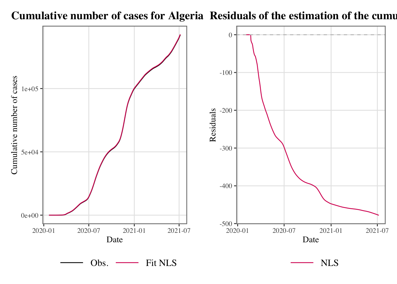
plot_fit <- function(country) {
  resul_country <-resul_fit_countries[[country]] 
  dat_country <- resul_country$dat
  
  dat_country <- 
    dat_country |> 
    mutate(
      fit_nls = resul_country$nls$fit
    )
  
  # Obs and fitted values
  p_1 <- 
    ggplot(
      data = dat_country |> 
        select(date, C_m, fit_nls) |> 
        pivot_longer(cols = c(C_m, fit_nls)) |> 
        mutate(
          name = factor(
            name,
            levels = c("C_m", "fit_nls"),
            labels = c("Obs.", "Fit NLS")
          )
        ),
      mapping = aes(x = date, y = value, colour = name)
    ) +
    geom_line() +
    scale_colour_manual(
      NULL,
      values = c("Obs." = "black", "Fit NLS" = "#D81B60")
    ) +
    labs(
      x = "Date", y = "Cumulative number of cases",
      title = str_c("Cumulative number of cases for ", country)
    ) +
    theme_paper() +
    theme(
      legend.key.height = unit(1, "line"),
      legend.key.width  = unit(2.5, "line"),
      legend.box = "horizontal"
    ) +
    guides(colour = guide_legend(override.aes = list(size = 1.8)))
  
  # Residuals
  p_2 <- 
    ggplot(
      data = dat_country |> 
        select(date, C_m, fit_nls) |> 
        pivot_longer(cols = c(fit_nls)) |> 
        mutate(error = C_m - value) |> 
        mutate(
          name = factor(
            name,
            levels = c("fit_nls"),
            labels = c("NLS")
          )
        ),
      mapping = aes(x = date, y = error, colour = name)
    ) +
    geom_line() +
    geom_hline(yintercept = 0, linetype = "dashed", colour = "grey") +
    scale_colour_manual(NULL, values = c("NLS" = "#D81B60")) +
    labs(
      x = "Date", y = "Residuals",
      title = str_c(
        "Residuals of the estimation of the cumulative number of cases for ",
        country
      )
    ) +
    theme_paper() +
    theme(
      legend.key.height = unit(1, "line"),
      legend.key.width  = unit(2.5, "line"),
      legend.box = "horizontal"
    ) +
    guides(colour = guide_legend(override.aes = list(size = 1.8)))
  
  cowplot::plot_grid(p_1, p_2)
}

plot_fit("Algeria")

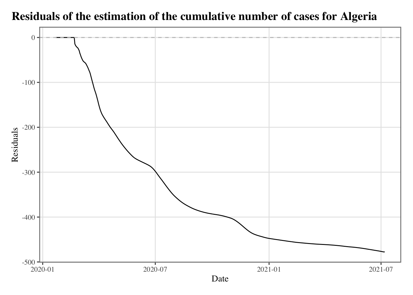
Let us focus on the residuals:

plot_fit_2 <- function(country) {
  resul_country <-resul_fit_countries[[country]] 
  dat_country <- resul_country$dat
  
  dat_country <- 
    dat_country |> 
    mutate(fit_nls = resul_country$nls$fit)
  
  # Residuals
  p_2 <- 
    ggplot(
      data = dat_country |> 
        select(date, C_m, fit_nls) |> 
        pivot_longer(cols = c(fit_nls)) |> 
        mutate(error = C_m - value),
      mapping = aes(x = date, y = error)) +
    geom_line() +
    geom_hline(yintercept = 0, linetype = "dashed", colour = "grey") +
    scale_colour_manual(NULL, values = c("NLS" = "#D81B60")) +
    labs(
      x = "Date", y = "Residuals",
      title = str_c("Residuals of the estimation of the cumulative number of cases for ",country)
    ) +
    theme_paper() +
    theme(
      legend.key.height = unit(1, "line"),
      legend.key.width  = unit(2.5, "line"),
      legend.box = "horizontal") +
    guides(colour = guide_legend(override.aes = list(size = 1.8)))
  
  p_2
}

plot_fit_2("Algeria")

4.2 Descriptive Statistics of the Estimates

estimates_all <- 
  estimates_nls |> 
  left_join(list_countries, by = "country")

library(kableExtra)

Attaching package: 'kableExtra'

The following object is masked from 'package:dplyr':

    group_rows

# All countries
results_desc_stat_all <- 
  estimates_all |> 
  mutate(estim = factor(estim, levels = c("nls"))) |> 
  pivot_longer(cols = c(r, P, alpha, K), names_to = "coef_name") |> 
  mutate(coef_name = factor(coef_name, levels = c("r", "P", "alpha", "K"))) |> 
  mutate(group = "All countries") |> 
  group_by(estim, group, coef_name) |> 
  summarise(
    Min = min(value),
    Max = max(value),
    Q1 = quantile(value, probs = 0.25),
    Median = median(value),
    Q3 = quantile(value, probs = 0.75),
    Mean = mean(value),
    `Standard Error` = sd(value),
    n = n()
  ) |> 
  pivot_longer(cols = Min:n, names_to = "stat_name") |> 
  pivot_wider(names_from = c(estim, coef_name), values_from = value)

`summarise()` has grouped output by 'estim', 'group'. You can override using
the `.groups` argument.

results_desc_stat_groups <- 
  estimates_all |> 
  mutate(
    estim = factor(estim, levels = c("nls")),
    group = factor(
      group, 
      levels = c("MENA", "Sub-Saharan Africa", "Asia", "Latin America", 
                 "Industrialized")
    )
  ) |> 
  pivot_longer(cols = c(r, P, alpha, K), names_to = "coef_name") |> 
  mutate(coef_name = factor(coef_name, levels = c("r", "P", "alpha", "K"))) |> 
  group_by(estim, group, coef_name) |> 
  summarise(
    Min = min(value),
    Max = max(value),
    Q1 = quantile(value, probs = 0.25),
    Median = median(value),
    Q3 = quantile(value, probs = 0.75),
    Mean = mean(value),
    `Standard Error` = sd(value),
    n = n()
  ) |> 
  pivot_longer(cols = Min:n, names_to = "stat_name") |> 
  pivot_wider(names_from = c(estim, coef_name), values_from = value)

`summarise()` has grouped output by 'estim', 'group'. You can override using
the `.groups` argument.

results_desc_stat <- 
  results_desc_stat_all |> 
  bind_rows(results_desc_stat_groups) |> 
  mutate(
    group = factor(
      group,
      levels = c("All countries", "MENA", "Sub-Saharan Africa", "Asia", 
                 "Latin America", "Industrialized")
    )
  ) |> 
  ungroup()

names(results_desc_stat) <- str_replace(
  names(results_desc_stat), "(^nls_)", ""
)

results_desc_stat <- 
  results_desc_stat |> 
  pivot_longer(cols = c(r, P, alpha, K)) |> 
  pivot_wider(names_from = stat_name, values_from = value) |> 
  mutate(name = factor(name, levels = c("r", "P", "alpha", "K"))) |> 
  arrange(name, group)

kableExtra::kable(
  results_desc_stat |> select(-name),
  caption = "Descriptive statistics of the estimates of the Parameters of Generalized Richards model.",
  booktabs = TRUE,
  digits = 2
) |> 
  pack_rows(index = table(fct_inorder(results_desc_stat$name))) |> 
  kableExtra::kable_styling() |>
  kableExtra::scroll_box(width = "100%", box_css = "border: 0px;")

Descriptive statistics of the estimates of the Parameters of Generalized Richards model.

group	Min	Max	Q1	Median	Q3	Mean	Standard Error	n
r
All countries	0.00	1.000000e+02	0.06	19.58	46.41	26.23	27.90	115
MENA	0.01	5.347000e+01	8.38	23.01	42.51	25.23	20.04	16
Sub-Saharan Africa	0.00	8.657000e+01	0.01	0.04	22.27	12.10	19.70	42
Asia	0.01	1.000000e+02	0.93	8.22	32.88	19.86	26.11	23
Latin America	0.00	1.000000e+02	12.09	47.37	55.99	38.84	27.79	18
Industrialized	0.12	1.000000e+02	45.53	56.17	79.68	59.33	24.44	16
P
All countries	0.00	1.000000e+00	0.36	0.46	0.90	0.57	0.29	115
MENA	0.29	1.000000e+00	0.35	0.37	0.46	0.49	0.25	16
Sub-Saharan Africa	0.16	1.000000e+00	0.30	0.95	1.00	0.70	0.34	42
Asia	0.00	1.000000e+00	0.44	0.61	0.74	0.60	0.26	23
Latin America	0.21	1.000000e+00	0.31	0.40	0.53	0.45	0.19	18
Industrialized	0.37	8.200000e-01	0.39	0.42	0.45	0.45	0.10	16
alpha
All countries	0.00	2.682000e+01	0.09	0.15	3.48	2.50	4.49	115
MENA	0.02	1.392000e+01	0.14	0.16	6.08	2.87	4.31	16
Sub-Saharan Africa	0.00	2.682000e+01	0.15	2.44	5.52	4.16	6.13	42
Asia	0.00	7.250000e+00	0.02	0.06	3.23	1.52	2.42	23
Latin America	0.00	9.170000e+00	0.04	0.14	2.20	1.50	2.55	18
Industrialized	0.04	3.450000e+00	0.11	0.12	0.14	0.32	0.83	16
K
All countries	0.00	1.394874e+09	699453.96	10166566.20	42585176.30	57005096.26	184880911.06	115
MENA	6824.55	8.435678e+07	2354827.40	7407575.70	34558098.05	17824805.48	23284286.06	16
Sub-Saharan Africa	1865.80	1.935701e+08	15292.39	2164900.32	17107419.65	18074630.53	36981678.01	42
Asia	0.00	1.394874e+09	2170264.80	35697881.40	125541489.80	176102231.72	385113433.97	23
Latin America	61154.19	2.085004e+08	4660258.90	13760635.60	31303437.40	32291527.27	52686073.88	18
Industrialized	29362.36	3.248202e+08	9729979.20	26870197.60	66249338.55	54978492.49	80354026.96	16

4.2.1 Comparison with and without Sub-Saharan Africa

# All countries
results_desc_stat_all <- 
  estimates_nls |> 
  mutate(estim = factor(estim, levels = c("nls"))) |> 
  pivot_longer(cols = c(r, P, alpha, K), names_to = "coef_name") |> 
  mutate(coef_name = factor(coef_name, levels = c("r", "P", "alpha", "K"))) |> 
  mutate(group = "All countries") |> 
  group_by(estim, group, coef_name) |> 
  summarise(
    Min = min(value),
    Max = max(value),
    Q1 = quantile(value, probs = 0.25),
    Median = median(value),
    Q3 = quantile(value, probs = 0.75),
    Mean = mean(value),
    `Standard Error` = sd(value),
    n = n()
  ) |> 
  pivot_longer(cols = Min:n, names_to = "stat_name") |> 
  pivot_wider(names_from = c(estim, coef_name), values_from = value)

`summarise()` has grouped output by 'estim', 'group'. You can override using
the `.groups` argument.

load("./data/output/list_countries.rda")

# All countries without SSA
results_desc_stat_wo_africa <- 
  estimates_nls |> 
  left_join(list_countries) |> 
  mutate(estim = factor(estim, levels = c("nls"))) |> 
  pivot_longer(cols = c(r, P, alpha, K), names_to = "coef_name") |> 
  mutate(coef_name = factor(coef_name, levels = c("r", "P", "alpha", "K"))) |> 
  filter(group != "Sub-Saharan Africa") |> 
  mutate(group = "All countries without S.-S. Africa") |> 
  group_by(estim, group, coef_name) |> 
  summarise(
    Min = min(value),
    Max = max(value),
    Q1 = quantile(value, probs = 0.25),
    Median = median(value),
    Q3 = quantile(value, probs = 0.75),
    Mean = mean(value),
    `Standard Error` = sd(value),
    n = n()
  ) |> 
  pivot_longer(cols = Min:n, names_to = "stat_name") |> 
  pivot_wider(names_from = c(estim, coef_name), values_from = value)

Joining with `by = join_by(country)`
`summarise()` has grouped output by 'estim', 'group'. You can override using
the `.groups` argument.

#  SSA
results_desc_stat_africa <- 
  estimates_nls |> 
  left_join(list_countries) |> 
  mutate(estim = factor(estim, levels = c("nls"))) |> 
  pivot_longer(cols = c(r, P, alpha, K), names_to = "coef_name") |> 
  mutate(coef_name = factor(coef_name, levels = c("r", "P", "alpha", "K"))) |> 
  filter(group == "Sub-Saharan Africa") |> 
  group_by(estim, group, coef_name) |> 
  summarise(
    Min = min(value),
    Max = max(value),
    Q1 = quantile(value, probs = 0.25),
    Median = median(value),
    Q3 = quantile(value, probs = 0.75),
    Mean = mean(value),
    `Standard Error` = sd(value),
    n = n()
  ) |> 
  pivot_longer(cols = Min:n, names_to = "stat_name") |> 
  pivot_wider(names_from = c(estim, coef_name), values_from = value)

Joining with `by = join_by(country)`
`summarise()` has grouped output by 'estim', 'group'. You can override using
the `.groups` argument.

results_desc_stat_2 <- 
  results_desc_stat_all |> 
  bind_rows(results_desc_stat_wo_africa) |> 
  bind_rows(results_desc_stat_africa) |> 
  mutate(
  group = factor(
    group,
    levels = c("All countries", "All countries without S.-S. Africa", "Sub-Saharan Africa")
  )
) |> 
  ungroup()

names(results_desc_stat_2) <- str_replace(
  names(results_desc_stat_2), "(^nls_)", ""
)

results_desc_stat_2 <- 
  results_desc_stat_2 |> 
  pivot_longer(cols = c(r, P, alpha, K)) |> 
  pivot_wider(names_from = stat_name, values_from = value) |> 
  mutate(name = factor(name, levels = c("r", "P", "alpha", "K"))) |> 
  arrange(name, group)

results_desc_stat_latex_2 <-
  results_desc_stat_2 |> 
  mutate(across(Min:`Standard Error`, ~ifelse(name == "K", yes = .x / 10^6, no = .x))) |> 
  relocate(name, .before = group)

kableExtra::kable(
  format = "html", 
  format.args = list(big.mark = ",", scientific = FALSE),
  results_desc_stat_latex_2[, -1],
  caption = "Descriptive statistics of the estimates of the Parameters of Generalized Richards model.",
  booktabs = TRUE,
  digits = 2
) |> 
  pack_rows(index = table(fct_inorder(results_desc_stat_latex_2$name))) |> 
  kableExtra::kable_styling() |>
  kableExtra::scroll_box(width = "100%", box_css = "border: 0px;")

Descriptive statistics of the estimates of the Parameters of Generalized Richards model.

group	Min	Max	Q1	Median	Q3	Mean	Standard Error	n
r
All countries	0.00	100.00	0.06	19.58	46.41	26.23	27.90	115
All countries without S.-S. Africa	0.00	100.00	6.08	36.40	53.47	34.37	28.78	73
Sub-Saharan Africa	0.00	86.57	0.01	0.04	22.27	12.10	19.70	42
P
All countries	0.00	1.00	0.36	0.46	0.90	0.57	0.29	115
All countries without S.-S. Africa	0.00	1.00	0.37	0.44	0.62	0.50	0.22	73
Sub-Saharan Africa	0.16	1.00	0.30	0.95	1.00	0.70	0.34	42
alpha
All countries	0.00	26.82	0.09	0.15	3.48	2.50	4.49	115
All countries without S.-S. Africa	0.00	13.92	0.06	0.13	1.98	1.55	2.84	73
Sub-Saharan Africa	0.00	26.82	0.15	2.44	5.52	4.16	6.13	42
K
All countries	0.00	1,394.87	0.70	10.17	42.59	57.01	184.88	115
All countries without S.-S. Africa	0.00	1,394.87	4.17	16.74	52.27	79.40	227.92	73
Sub-Saharan Africa	0.00	193.57	0.02	2.16	17.11	18.07	36.98	42

If we want to have a look at the distribution of the different estimates by geographical grouping, we can proceed as follows.

df_plot_density_estimates <- 
  estimates_all |> 
  pivot_longer(cols = c(r, P, alpha, K), names_to = "coef_name") |> 
  mutate(group = "All countries") |> 
  bind_rows(
    estimates_all |> 
      pivot_longer(cols = c(r, P, alpha, K), names_to = "coef_name")
  ) |> 
  mutate(
    coef_name = factor(
      coef_name,
      levels = c("r", "P", "alpha", "K"),
      labels = c("r", "P", "alpha", "K")),
    group = factor(
      group,
      levels = c("All countries", "MENA", "Sub-Saharan Africa", "Asia", 
                 "Latin America", "Industrialized"),
      labels = c("All countries", "MENA", "S.-S. Africa", "Asia", 
                 "Latin America", "Industrialized")
    )
  )

p_distrib_estimates_geo <- ggplot(
  data = df_plot_density_estimates,
  mapping = aes(x = value)
) +
  geom_histogram(mapping = aes(group = group)) +
  facet_grid(
    group~coef_name, 
    scales = "free", 
    labeller = labeller(coef_name = label_parsed)
  ) +
  theme_paper() +
  labs(
    x = NULL, y = "Count",
    title = "Distribution of estimated values by geographical grouping"
  )
p_distrib_estimates_geo

`stat_bin()` using `bins = 30`. Pick better value with `binwidth`.

ggsave(
  p_distrib_estimates_geo + labs(title = NULL),
  file = "./figs/distrib_estimates_nls_geo.pdf", width = 10, height = 12
)

`stat_bin()` using `bins = 30`. Pick better value with `binwidth`.

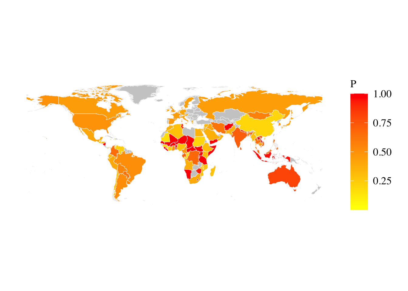
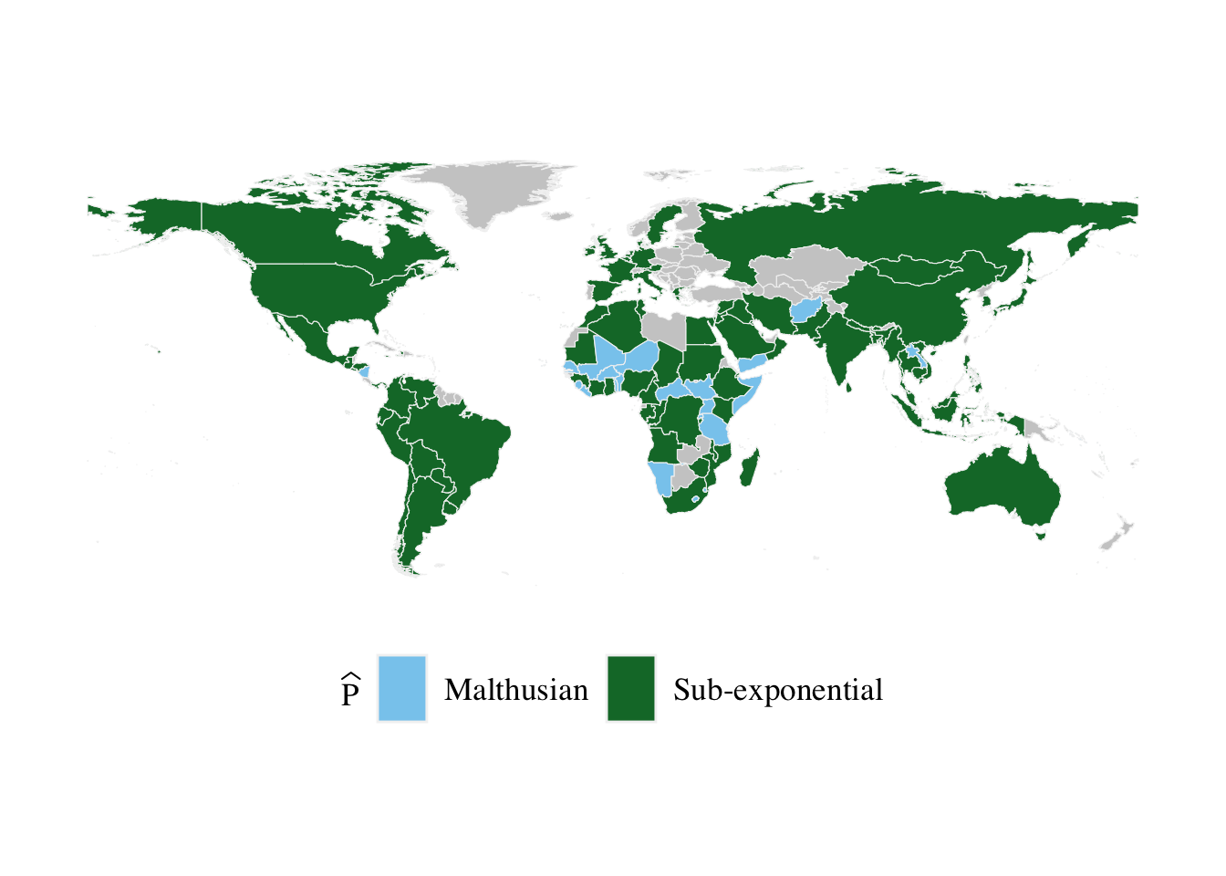
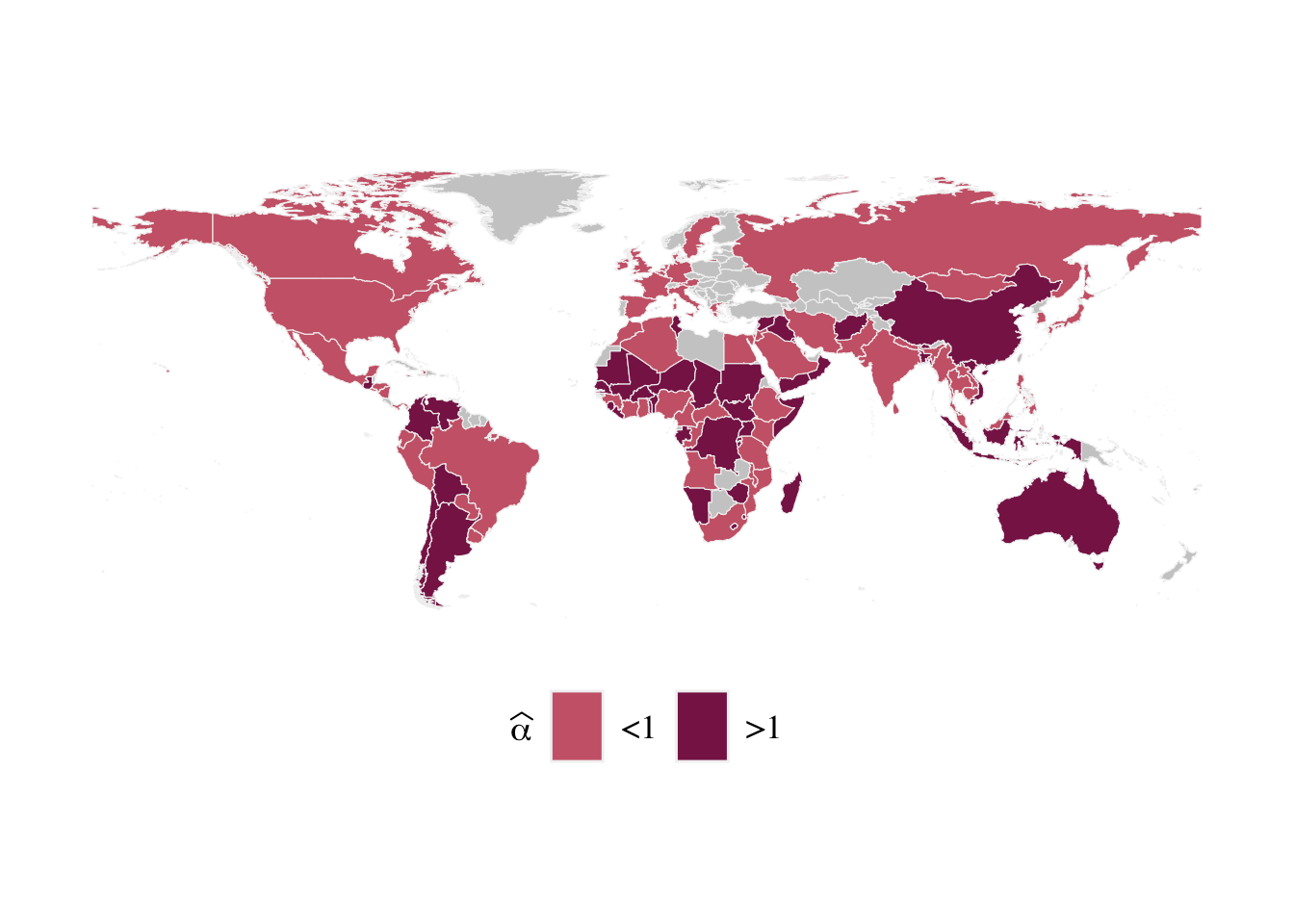
4.3 Maps

Let us define a theme for maps:

#' Theme for maps with ggplot2
#'
#' @param ... arguments passed to the theme function
#' @export
#' @importFrom ggplot2 element_rect element_text element_blank element_line unit
#'   rel
theme_map_paper <- function(...) {
  theme(
    text = element_text(family = "Times"),
    plot.background = element_rect(fill = "transparent", color = NA),
    panel.background = element_rect(fill = "transparent", color = NA),
    panel.border = element_blank(),
    axis.title = element_blank(),
    axis.text = element_blank(),
    axis.ticks = element_blank(), axis.line = element_blank(),
    plot.title.position = "plot",
    legend.text = element_text(size = rel(1.2)),
    legend.title = element_text(size = rel(1.2)),
    legend.background = element_rect(fill="transparent", color = NULL),
    legend.key = element_blank(),
    legend.key.height   = unit(2, "line"),
    legend.key.width    = unit(1.5, "line"),
    strip.background = element_rect(fill = NA),
    panel.spacing = unit(1, "lines"),
    panel.grid.major = element_blank(),
    panel.grid.minor = element_blank(),
    plot.margin = unit(c(1, 1, 1, 1), "lines"),
    strip.text = element_text(size = rel(1.2))
  )
}

A Shapefile that allows us to display the level 0 world administrative boundaries, freely available on the online open data platform “opendatasoft”, can be loaded:

library(sf)

Linking to GEOS 3.11.0, GDAL 3.5.3, PROJ 9.1.0; sf_use_s2() is TRUE

world_map <- sf::read_sf(
  "./data/raw/world-administrative-boundaries/world-administrative-boundaries.shp"
)

There are some mismatching country names between the map file and the epidemic data. The names from the map file can be manually changed:

world_map <- 
  world_map |> 
  mutate(
    name = recode(
      name, 
      # old = new
      "Brunei Darussalam" = "Brunei",
      "Côte d'Ivoire" = "Cote d'Ivoire",
      "Democratic Republic of the Congo" = "Democratic Republic of Congo",
      "Swaziland" = "Eswatini",
      "Iran (Islamic Republic of)" = "Iran",
      "Lao People's Democratic Republic" = "Laos",
      "Russian Federation" = "Russia",
      "Republic of Korea" = "South Korea",
      "Syrian Arab Republic" = "Syria",
      "United Republic of Tanzania" = "Tanzania",
      "U.K. of Great Britain and Northern Ireland" = "United Kingdom",
      "United States of America" = "United States"
    )
  )

Let us add the estimated values for each country to the map data:

map_nls <- 
  world_map |> 
  left_join(
    estimates_all |> 
      filter(estim == "nls"),
    by = c("name" = "country")
  )

ggplot(data = map_nls) +
  geom_sf(mapping = aes(fill = P), colour = "gray95", size = .1) +
  scale_fill_gradient(low = "yellow", high = "red", na.value = "gray80") +
  theme_map_paper()

Spatial distribution of estimated values for P by countries (NLS).

map_nls_P <- 
  ggplot(
    data = map_nls |> 
      mutate(growth = ifelse(P < 1, "Sub-exponential", "Malthusian"))
  ) +
  geom_sf(mapping = aes(fill = growth), colour = "gray95", size = .1) +
  scale_fill_manual(
    expression(widehat(P)), 
    values = c("Sub-exponential" = "#117733", "Malthusian" = "#88CCEE"),
    na.value = "gray80"
  ) +
  theme_map_paper() +
  theme(legend.position = "bottom")
map_nls_P

Spatial distribution of estimated values for ˆP by countries (NLS).

ggsave(map_nls_P, file = "./figs/map_nls_P.png", width = 12, height = 6)

map_nls_alpha <- 
  ggplot(
    data = map_nls |> 
      mutate(val = ifelse(alpha < 1, "<1", ">1"))
  ) +
  geom_sf(mapping = aes(fill = val), colour = "gray95", size = .1) +
  scale_fill_manual(
    expression(widehat(alpha)), 
    values = c("<1" = "#CC6677", ">1" = "#882255"),
    na.value = "gray80"
  ) +
  theme_map_paper() +
  theme(legend.position = "bottom")
map_nls_alpha

Spatial distribution of estimated values for ˆP by countries (NLS).

ggsave(map_nls_alpha, file = "./figs/map_nls_alpha.png", width = 12, height = 6)

estimates_nls |> 
  left_join(list_countries) |> 
  pivot_longer(cols = c(r, P, alpha, K)) |> 
  group_by(name, group) |> 
  mutate(
    estim = factor(estim, levels = c("nls"),
                   labels = c("Non linear Least Square"))
  ) |> 
  filter(estim == "Non linear Least Square") |> 
  filter(name %in% c("alpha", "P")) |> 
  filter((name == "alpha" & value > 500))

Joining with `by = join_by(country)`

# A tibble: 0 × 5
# Groups:   name, group [0]
# ℹ 5 variables: country <chr>, estim <fct>, group <chr>, name <chr>,
#   value <dbl>

p_nls_alpha_P <- 
  ggplot(
    data = estimates_nls |> 
      left_join(list_countries) |> 
      pivot_longer(cols = c(r, P, alpha, K)) |> 
      group_by(name, group) |> 
      mutate(
        estim = factor(estim, levels = c("nls"),
                       labels = c("Non linear Least Square"))
      ) |> 
      filter(estim == "Non linear Least Square") |> 
      filter(name %in% c("alpha", "P")) |> 
      filter(!(name == "alpha" & value > 500)) |> 
      mutate(
        name = factor(
          name,
          levels = c("P", "alpha"),
          labels = c(expression(hat(P)), expression(hat(alpha)))
        )
      ) |> 
      mutate(
        group = factor(
          group,
          levels = c("MENA", "Sub-Saharan Africa", "Latin America", "Asia", 
                     "Industrialized")
        )
      )
  ) +
  geom_boxplot(aes(x = estim, y = value), na.rm = TRUE) +
  facet_grid(name~group, scales = "free", labeller = labeller(type = label_parsed)) + 
  labs(x = NULL, y = "Estimate",
       title = "Estimated coefficients for the Generalized Richards Model") +
  theme_paper() +
  theme(axis.text.x=element_blank())

Joining with `by = join_by(country)`

p_nls_alpha_P

ggsave(
  p_nls_alpha_P + labs(title = NULL),
  file = "./figs/p_nls_alpha_P.pdf", width = 12, height = 6
)