3  Principal Component Analysis

Some packages are needed:

library(tidyverse)
── Attaching core tidyverse packages ──────────────────────── tidyverse 2.0.0 ──
✔ dplyr     1.1.3     ✔ readr     2.1.4
✔ forcats   1.0.0     ✔ stringr   1.5.0
✔ ggplot2   3.4.4     ✔ tibble    3.2.1
✔ lubridate 1.9.3     ✔ tidyr     1.3.0
✔ purrr     1.0.2     
── Conflicts ────────────────────────────────────────── tidyverse_conflicts() ──
✖ dplyr::filter() masks stats::filter()
✖ dplyr::lag()    masks stats::lag()
ℹ Use the conflicted package (<http://conflicted.r-lib.org/>) to force all conflicts to become errors
library(FactoMineR)
library(factoextra)
Welcome! Want to learn more? See two factoextra-related books at https://goo.gl/ve3WBa
library(ggcorrplot)
library(stats)
library(knitr)
library(rmarkdown) 
library(kableExtra)

Attaching package: 'kableExtra'

The following object is masked from 'package:dplyr':

    group_rows
library(DT)

3.1 Load data

load("./data/output/covid/df_all_countries.rda")
df_all_covid
# A tibble: 115 × 88
   country type_Air transport, p…¹ type_Diabetes preval…² type_Domestic genera…³
   <chr>   <chr>                   <chr>                  <chr>                 
 1 Algeria value 2020              last 10                value 2020            
 2 Bahrain value 2020              last 10                value 2020            
 3 Egypt   value 2020              last 10                value 2020            
 4 Iran    value 2020              last 10                value 2020            
 5 Iraq    value 2020              last 10                value 2020            
 6 Israel  value 2020              last 10                value 2020            
 7 Jordan  value 2020              last 10                value 2020            
 8 Kuwait  value 2020              last 10                value 2020            
 9 Lebanon value 2020              last 10                value 2020            
10 Morocco value 2020              last 10                value 2020            
# ℹ 105 more rows
# ℹ abbreviated names: ¹​`type_Air transport, passengers carried`,
#   ²​`type_Diabetes prevalence (% of population ages 20 to 79)`,
#   ³​`type_Domestic general government health expenditure (% of general government expenditure)`
# ℹ 84 more variables:
#   `type_Domestic private health expenditure per capita (current US$)` <chr>,
#   `type_Domestic private health expenditure per capita, PPP (current international $)` <chr>, …

Let us check if there are duplicate countries:

sum(duplicated(df_all_covid))
[1] 0

3.2 Principal Component Analysis

Let us define a function to perform a principal component analysis. It allows us to obtain the coordinates weighted by the eigenvalues for each factor S1, S2, S3, S4, S5, S6.

#' Performs PCA on a group of variables (S1, S2, S3, S4, S5, or S6)
#' 
#' @param variables_to_keep group of variables concerned
#' @param type (string) name of group of variables
get_res_acp <- function(variables_to_keep, type) {
  
  # Keep only the variables considered in the database
  df_acp <- 
    df_all_covid |> 
    select(country, str_c("value_", variables_to_keep)) |> 
    rename_with(~str_remove(., "^value_"))
  
  # Take Country name like row_name
  df_acp <- data.frame(df_acp, row.names = 1, check.names = F)
  
  # PCA
  pca_res <- PCA(
    df_acp,
    graph = FALSE,
    scale.unit = TRUE,
    ncp = length(variables_to_keep)
  )
  
  # Obtain the coordinate of individuals
  ind_data <- get_pca_ind(pca_res)
  ind_coord <- data.frame(ind_data$coord)
  
  # Obtain the proportion of eigenvalues relating to each factor
  eigen <- get_eigenvalue(pca_res)
  weights <- data.frame(eigen[,2]/100)
  
  # Coordinates
  df_coord <- data.frame(crossprod(t(ind_coord),weights[,1]))
  df_coord <- df_coord |>
    mutate(country = rownames(df_coord))
  rownames(df_coord) <- NULL
  
  names(df_coord) <- c(paste("coordinate",type,sep ="_"),"country")
  
  names(weights) <- "prop_var_expl"
  rownames(weights) <- NULL
  weights <- weights |> mutate(dim = row_number())
  
  list(
    coord = df_coord,
    weights = weights
  )
  
  
} # End of get_res_acp

3.2.1 S1: healthcare infrastructure

variables_to_keep <- c(
  "Physicians (per 1,000 people)",
  "Hospital beds (per 1,000 people)",
  "Nurses and midwives (per 1,000 people)",
  "Domestic general government health expenditure (% of general government expenditure)",
  "Domestic private health expenditure per capita (current US$)",
  "Domestic private health expenditure per capita, PPP (current international $)"
)

pca_s1 <- get_res_acp(
  variables_to_keep = variables_to_keep,
  type = "s1"
)

df_coordinate_s1 <- pca_s1$coord
prop_var_expl_s1 <- pca_s1$weights

3.2.2 S2: vulnerability to comorbidities

variables_to_keep <- c(
  "Incidence of malaria (per 1,000 population at risk)",
  "Incidence of HIV, all (per 1,000 uninfected population)",
  "Incidence of tuberculosis (per 100,000 people)",
  "Diabetes prevalence (% of population ages 20 to 79)",
  "Mortality from CVD, cancer, diabetes or CRD between exact ages 30 and 70 (%)"
  )

pca_s2 <- get_res_acp(
  variables_to_keep = variables_to_keep,
  type = "s2"
)

df_coordinate_s2 <- pca_s2$coord
prop_var_expl_s2 <- pca_s2$weights

3.2.3 S3: Vulnerability to natural environment

variables_to_keep <- c(
  "Mortality rate attributed to household and ambient air pollution, age-standardized (per 100,000 population)",
  "PM2.5 air pollution, mean annual exposure (micrograms per cubic meter)",
  "PM2.5 pollution, population exposed to levels exceeding WHO Interim Target-1 value (% of total)",
  "PM2.5 pollution, population exposed to levels exceeding WHO Interim Target-2 value (% of total)",
  "PM2.5 pollution, population exposed to levels exceeding WHO Interim Target-3 value (% of total)",
  "Air transport, passengers carried",
  "International tourism, number of arrivals",
  "Ecological Footprint")


pca_s3 <- get_res_acp(
  variables_to_keep = variables_to_keep,
  type = "s3"
)

df_coordinate_s3 <- pca_s3$coord
prop_var_expl_s3 <- pca_s3$weights

3.2.4 S4: Living conditions

variables_to_keep <- c(
  "People using at least basic drinking water services (% of population)",
  "People using at least basic sanitation services (% of population)",
  "Prevalence of undernourishment (% of population)",
  "Prevalence of anemia among women of reproductive age (% of women ages 15-49)",
  "Poverty headcount ratio at $3.65 a day (2017 PPP) (% of population)",
  "Poverty headcount ratio at $6.85 a day (2017 PPP) (% of population)",
  "Poverty headcount ratio at national poverty lines (% of population)",
  "GDP per capita (current US$)",
  "GDP per capita, PPP (current international $)",
  "Urban density"
  )

pca_s4 <- get_res_acp(
  variables_to_keep = variables_to_keep,
  type = "s4"
)

df_coordinate_s4 <- pca_s4$coord
prop_var_expl_s4 <- pca_s4$weights

3.2.5 S5: Economic and societal characteristics

variables_to_keep <- c(
  "Population, total",
  "GDP per capita growth (annual %)",
  "International migrant stock (% of population)",
  "Population ages 65 and above (% of total population)",
  "Individuals using the Internet (% of population)",
  "Mobile cellular subscriptions (per 100 people)",
  "Shadow size Economy",
  "Gini index (CIA estimate)"
)

pca_s5 <- get_res_acp(
  variables_to_keep = variables_to_keep,
  type = "s5"
)

df_coordinate_s5 <- pca_s5$coord
prop_var_expl_s5 <- pca_s5$weights

3.2.6 S6: Policy variables

variables_to_keep <- c(
  "GovernmentResponseIndex",                                                   
  "ContainmentHealthIndex",           
  "StringencyIndex",                                    
  "EconomicSupportIndex"
)

pca_s6 <- get_res_acp(
  variables_to_keep = variables_to_keep,
  type = "s6"
)

df_coordinate_s6 <- pca_s6$coord
prop_var_expl_s6 <- pca_s6$weights

3.2.7 Final table containing all the coordianetes

load("./data/output/list_countries.rda")
df_coordinates <- 
  df_coordinate_s1 |> 
  merge(df_coordinate_s2) |> 
  merge(df_coordinate_s3) |> 
  merge(df_coordinate_s4) |> 
  merge(df_coordinate_s5) |> 
  merge(df_coordinate_s6) |> 
  left_join(list_countries, by = "country")

write_excel_csv(
  df_coordinates,
  file = "./estim/results_pca/df_coordinates.csv"
)
df_coordinates
                         country coordinate_s1 coordinate_s2 coordinate_s3
1                    Afghanistan   -1.21862387   0.585556190   1.468395696
2                        Algeria   -0.21659429  -0.610474440   0.441892918
3                         Angola   -1.18481459   0.695112791   0.356279120
4                      Argentina    1.32352447  -0.593971671  -1.264056359
5                      Australia    2.88084417  -0.948890170  -1.512026190
6                        Austria    3.16206730  -0.854782998  -1.414217706
7                        Bahrain   -0.02925388  -0.291208694   0.814800849
8                     Bangladesh   -1.19133172  -0.007618773   1.225790522
9                        Belgium    2.52610326  -0.893179082  -1.456893848
10                         Benin   -1.32964814   0.228730643   0.864140926
11                        Bhutan   -0.61470218  -0.219402561   0.456844652
12                       Bolivia   -0.35290142  -0.333498120  -0.428982472
13                        Brazil    0.85001831  -0.426444842  -1.172810347
14                        Brunei   -0.02318024  -0.299477388  -1.564960601
15                  Burkina Faso   -0.99780444   0.276220215   1.250252228
16                       Burundi   -1.11003420   0.322473897   1.053216925
17                      Cambodia   -0.98196013   0.107113208   0.002055174
18                      Cameroon   -1.18369764   0.564011811   1.398047830
19                        Canada    2.25500780  -0.848947543  -1.615274252
20                    Cape Verde   -0.55209542  -0.548212538   0.554854717
21      Central African Republic   -1.24220390   1.886983211   1.481777623
22                          Chad   -1.34706341   0.228819724   1.400944989
23                         Chile    1.15047465  -0.737020429  -0.713203077
24                         China    0.30308729  -0.460350982   1.735654891
25                      Colombia    0.26863282  -0.711713502  -0.908090284
26                         Congo   -0.90584615   1.410850823   0.986983041
27                 Cote d'Ivoire   -1.16564784   0.303119594   0.542043480
28  Democratic Republic of Congo   -1.08474793   0.760757970   1.043918983
29                       Denmark    1.99081221  -0.871072843  -1.481692227
30                      Djibouti   -1.13794396   0.198000114   1.049881758
31                       Ecuador    0.07366003  -0.733304723  -1.030438549
32                         Egypt   -0.69668891   0.163103150   1.124555030
33                   El Salvador    0.10110623  -0.670216668  -0.463673449
34                      Eswatini   -0.56685921   2.978021294  -0.299418781
35                      Ethiopia   -1.23508467  -0.322378032   0.732459929
36                        France    2.66037328  -0.875786656  -1.554939742
37                         Gabon    0.22503829   1.269753294   0.668726967
38                        Gambia   -1.15585941   0.092117880   1.019831729
39                       Germany    3.80212023  -0.836960913  -1.410873930
40                         Ghana   -0.85738279   0.309142740   0.916442692
41                        Greece    1.80856324  -0.823598220  -1.087022962
42                     Guatemala   -0.24062878  -0.499572923  -0.309015149
43                        Guinea   -1.27477590   0.665215950   0.554022821
44                         Haiti   -1.29380792   0.460883859  -0.480918641
45                      Honduras   -0.69867527  -0.435160405  -0.408769397
46                         India   -1.10622365   0.085402926   1.469495893
47                     Indonesia   -0.52420295   0.319112621  -0.704069192
48                          Iran    0.28382192  -0.560077572   0.357599198
49                          Iraq   -0.66896317  -0.209022684   0.863695235
50                       Ireland    2.66461955  -0.919187619  -1.443407535
51                        Israel    1.48686182  -0.923407264  -0.821948818
52                         Italy    1.46842207  -0.970042038  -1.124883252
53                       Jamaica   -0.42969015  -0.267339948  -1.245495733
54                         Japan    3.56451464  -0.917888619  -1.310819039
55                        Jordan    0.05219600  -0.548716511   0.005303699
56                         Kenya   -0.92436206   0.295759495   0.061788483
57                        Kuwait    0.27669178  -0.451639175   0.764844020
58                          Laos   -1.00911260   0.043720502   0.052629053
59                       Lebanon    0.57454989  -0.127775333  -0.065725895
60                       Lesotho   -0.59499964   3.024188718   0.666433474
61                       Liberia   -1.22125077   0.776562132  -0.017227459
62                    Madagascar   -1.18909178   0.480425188  -0.143730684
63                        Malawi   -0.99883391   0.544907953  -0.254481655
64                      Malaysia    0.09397601  -0.219107057  -0.871377351
65                          Mali   -1.34999751   0.213429340   1.054681508
66                    Mauritania   -1.14039635  -0.456739466   1.179732513
67                     Mauritius    0.57181405   0.009687679  -1.050236105
68                        Mexico    0.05105243  -0.369969351  -0.650952921
69                      Mongolia    1.04117250   1.032345478   0.620935940
70                       Morocco   -0.77608409  -0.112806187   0.139183519
71                    Mozambique   -1.18174367   1.360376633  -0.093608725
72                       Myanmar   -1.02845848   0.426487717   0.620896170
73                       Namibia   -0.16850028   1.370349367  -0.019062420
74                         Nepal   -0.89140826  -0.027405485   1.554013334
75                   Netherlands    3.08628392  -0.910929944  -1.487755168
76                     Nicaragua   -0.26874709  -0.454698331  -0.689210150
77                         Niger   -1.12463914   0.152470569   1.612044185
78                       Nigeria   -1.00224120   0.368771740   1.261786625
79                          Oman   -0.20051581  -0.264041926   0.737612306
80                      Pakistan   -1.07258437   0.500544603   1.360572785
81                        Panama    0.84731425  -0.695526889  -1.360748902
82                      Paraguay   -0.27113810  -0.537758504  -1.334467669
83                          Peru   -0.07332750  -0.658357330  -0.346023743
84                   Philippines   -0.42277515   0.881241610  -0.293422125
85                         Qatar    0.50511997  -0.457027863   0.994938380
86                        Russia    2.12861097  -0.058570769  -0.846309256
87                        Rwanda   -0.88616712  -0.028203215   0.962308276
88                  Saudi Arabia    0.72703455  -0.066280381   0.969485636
89                       Senegal   -1.26357911  -0.255767356   1.100739747
90                    Seychelles    0.63885892  -0.014355689  -0.771576379
91                  Sierra Leone   -1.26512653   0.801285524   0.264333743
92               Solomon Islands   -0.76265376   0.934950089  -0.641727470
93                       Somalia   -1.13811883   0.774193009   0.622413242
94                  South Africa    0.21052324   2.085008177  -0.258767421
95                   South Korea    3.18910163  -0.871220204  -0.391584077
96                   South Sudan   -1.34472667   0.519286474   0.872850966
97                         Spain    1.57996391  -0.890446000  -1.509234013
98                     Sri Lanka    0.01168562  -0.602700939  -0.640733623
99                         Sudan   -0.95027458  -0.063443118   1.075639966
100                       Sweden    2.10456255  -1.008366576  -1.591195727
101                        Syria   -0.81771758  -0.282453665   0.507701960
102                     Tanzania   -1.07979100   0.223795026   0.012844562
103                     Thailand   -0.18255675  -0.421787063  -0.231537275
104                  Timor-Leste   -0.07018220   0.458628791  -0.266206013
105                         Togo   -1.21908109   0.158139038   0.989155567
106                      Tunisia   -0.20420461  -0.517176134   0.356586030
107                       Uganda   -1.28691435   0.632719116   0.970965255
108               United Kingdom    1.68327867  -0.891418414  -1.452743602
109                United States    6.10722432  -0.654581306  -0.759984116
110                      Uruguay    1.62895570  -0.520655825  -1.489792336
111                      Vanuatu   -0.76869596   0.687236467  -0.718336749
112                    Venezuela   -0.65083268  -0.429608837  -0.840063188
113                      Vietnam   -0.34485091  -0.155731081   0.152239524
114                        Yemen   -1.25095179   0.045044565   1.126789054
115                     Zimbabwe   -0.94407305   0.933417874  -0.190331594
    coordinate_s4 coordinate_s5 coordinate_s6              group
1     1.270616306  -0.956087817   -1.78989270               Asia
2    -1.099269663  -0.030008599    0.54343719               MENA
3     1.647035211  -0.881227673   -0.24910732 Sub-Saharan Africa
4    -1.115314454   0.644888636    2.44016976      Latin America
5    -2.383808110   0.745966967    1.14501180     Industrialized
6    -2.353472919   0.904544775    0.98979909     Industrialized
7    -1.146740332   0.649394318    1.65896777               MENA
8     0.312649160  -0.369105406    1.13743429               Asia
9    -2.365885257   0.678052413    1.00012446     Industrialized
10    1.684840654  -0.651092587   -1.05432610 Sub-Saharan Africa
11   -0.358015464   0.173132603    1.60272883               Asia
12   -0.232227870  -0.121553459    0.81515639      Latin America
13   -1.017579046   0.228588359    0.55889425      Latin America
14   -1.492464017   0.444580939   -0.78513346               Asia
15    2.193489495  -0.638172933   -2.23807144 Sub-Saharan Africa
16    2.264123144  -1.139977037   -4.53103218 Sub-Saharan Africa
17    0.072078349   0.037628251   -1.85818636               Asia
18    1.158591494  -0.472624402   -1.52087304 Sub-Saharan Africa
19   -2.228902185   0.617888729    0.72272782     Industrialized
20    0.158617858   0.090149618    1.39362807 Sub-Saharan Africa
21    3.680644147  -1.288581617   -1.60485963 Sub-Saharan Africa
22    2.532982648  -1.067827522   -0.05576503 Sub-Saharan Africa
23   -1.828215023   0.697298492    1.86045159      Latin America
24   -1.776040270   0.700821307    1.14166599               Asia
25   -0.239134657   0.452552046    1.77454870      Latin America
26    2.299780218  -0.568763109   -0.89574967 Sub-Saharan Africa
27    1.301393281   0.067436911   -0.98212331 Sub-Saharan Africa
28    3.549736293  -1.071427390   -1.16041293 Sub-Saharan Africa
29   -2.486155044   0.920896832    0.35853069     Industrialized
30    1.106655889  -0.681762414   -1.18915901 Sub-Saharan Africa
31   -0.472886893   0.020807688    1.31776975      Latin America
32   -0.565544017  -0.240703645    0.75673958               MENA
33   -0.974746300   0.463788440    1.72754181      Latin America
34    1.105038346  -0.150098011   -0.29977715 Sub-Saharan Africa
35    1.794676038  -1.218940592   -0.11301799 Sub-Saharan Africa
36   -2.240418995   0.867108732    1.12897877     Industrialized
37    0.478727364   0.241972438    1.91356881 Sub-Saharan Africa
38    1.633786787  -0.454456211   -0.92791004 Sub-Saharan Africa
39   -2.340559288   1.051280719    0.34189509     Industrialized
40    0.566707213  -0.013256653   -1.27039523 Sub-Saharan Africa
41   -1.751206288   0.779346194    1.09145584     Industrialized
42    0.204437579  -0.114211417    1.17711210      Latin America
43    1.760430092  -0.528130426   -0.16055964 Sub-Saharan Africa
44    2.697248573  -0.714936752   -0.98071342      Latin America
45    0.102386436  -0.496816623    2.29154077      Latin America
46    0.624536416   0.035788998    1.86728533               Asia
47   -0.679892066   0.200197683   -0.21010698               Asia
48   -1.060933514   0.452397899   -0.47086087               MENA
49   -0.802363699  -0.284842255    1.00736056               MENA
50   -2.721202484   0.482361539    1.59638669     Industrialized
51   -2.001743702   0.870787423    1.88794981               MENA
52   -2.025659701   0.964514216    1.65296235     Industrialized
53   -0.939041927   0.174933994    1.11666950      Latin America
54   -2.032987675   1.477237670   -0.48787626     Industrialized
55   -0.858374611  -0.114236795    0.25180997               MENA
56    1.752849789  -0.336352448    0.26512649 Sub-Saharan Africa
57   -1.377016418   1.177259814    0.85056157               MENA
58   -0.002582404  -0.593987851   -1.04678699               Asia
59   -1.019267466   0.392570120    0.64169943               MENA
60    1.632755477  -0.536044377   -0.99049266 Sub-Saharan Africa
61    2.320329624  -1.091453931   -1.00888416 Sub-Saharan Africa
62    3.661218992  -0.924884100   -0.59626965 Sub-Saharan Africa
63    1.890424263  -1.024593786   -0.09094998 Sub-Saharan Africa
64   -1.447965178   0.556810055    1.53164167               Asia
65    1.406402040  -0.319684064   -1.27816560 Sub-Saharan Africa
66    0.794704056  -0.007537122   -1.58269194 Sub-Saharan Africa
67   -1.582478225   0.715289041   -1.38293782 Sub-Saharan Africa
68   -0.780187287   0.122726541   -0.22062450      Latin America
69   -0.479011234   0.215896184    1.10315078               Asia
70   -0.788295982   0.499610544    1.32096869               MENA
71    2.588289017  -1.019745949   -1.01571891 Sub-Saharan Africa
72    0.125630020   0.059634631    0.50081621               Asia
73    0.256657222   0.044074568   -1.18889175 Sub-Saharan Africa
74    0.049925091   0.028402292    1.22309754               Asia
75   -2.389031052   0.898732240    0.68303725     Industrialized
76   -0.183019461  -0.311023566   -4.70602120      Latin America
77    2.464282831  -1.013991893   -3.11752960 Sub-Saharan Africa
78    1.543167751  -0.317338952   -0.10148203 Sub-Saharan Africa
79   -1.039518089   0.689336932    1.41983423               MENA
80    0.460443620  -0.696137644    0.70036472               Asia
81   -1.253938906   0.643978391    1.48594875      Latin America
82   -0.988941334   0.179450065    1.32007602      Latin America
83   -0.314590375   0.260196410    2.13402399      Latin America
84   -0.669668018   0.177593767    1.35706450               Asia
85   -1.732903821   0.892153709    0.99865026               MENA
86   -1.696535435   1.014755234    0.17776235               Asia
87    1.528193863  -0.629461476    1.54897884 Sub-Saharan Africa
88   -1.314446089   0.545867092    1.00917132               MENA
89    1.029867325  -0.215510766   -0.56693515 Sub-Saharan Africa
90   -0.916811982   0.901517082   -1.29205325 Sub-Saharan Africa
91    2.491478435  -0.731435221   -1.70525678 Sub-Saharan Africa
92    1.159273832  -0.661605582   -2.88865029               Asia
93    2.612177853  -1.188366653   -2.71760894 Sub-Saharan Africa
94    0.255176931   0.715394984    1.07177449 Sub-Saharan Africa
95   -1.986137486   0.826742645    0.28257479               Asia
96    3.112659781  -1.321141003   -0.79940066 Sub-Saharan Africa
97   -1.906171934   0.978931617    1.26428935     Industrialized
98   -0.835448064   0.175100543   -0.07661764               Asia
99    1.498538282  -0.641717560   -0.80246654 Sub-Saharan Africa
100  -2.319758014   0.948317454   -0.01954782     Industrialized
101  -0.631594008  -0.463102256   -1.66056589               MENA
102   1.804449352  -0.740921852   -3.94905060 Sub-Saharan Africa
103  -1.560188402   0.902739099    0.56720207               Asia
104   1.464144824  -0.816505654   -1.43974554               Asia
105   1.981719351  -0.706650965   -0.66091727 Sub-Saharan Africa
106  -1.216346554   0.324986281   -0.21314936               MENA
107   1.600659477  -1.079593815    0.49195854 Sub-Saharan Africa
108  -2.162610258   0.993382334    1.77154328     Industrialized
109  -2.499358160   0.757034626    0.52383291     Industrialized
110  -1.410288218   0.726538019   -0.24067229      Latin America
111   0.098100137  -0.388019678   -2.32734831               Asia
112  -0.247859892  -0.469485661    1.11395568      Latin America
113  -1.501627388   0.409768568    0.50977609               Asia
114   2.610979598  -0.862479280   -3.55365376               MENA
115   1.448674781  -0.533521259   -0.06218858 Sub-Saharan Africa

Let us normalise the scores:

df_coordinates <- 
  df_coordinates |> 
  pivot_longer(cols = coordinate_s1:coordinate_s6, values_to = "coord") |> 
  group_by(name) |> 
  mutate(coord_norm = (coord - min(coord)) / (max(coord) - min(coord))) |> 
  mutate(name = str_remove(name, "coordinate_")) |> 
  pivot_wider(values_from = c(coord, coord_norm), names_from = name)

save(df_coordinates, file = "./estim/results_pca/df_coordinates.rda")
prop_var_expl <- 
  prop_var_expl_s1 |> 
  mutate(type = "s1") |> 
  bind_rows(
    prop_var_expl_s2 |> mutate(type = "s2")
  ) |> 
  bind_rows(
    prop_var_expl_s3 |> mutate(type = "s3")
  ) |> 
  bind_rows(
    prop_var_expl_s4 |> mutate(type = "s4")
  ) |> 
  bind_rows(
    prop_var_expl_s5 |> mutate(type = "s5")
  ) |> 
  bind_rows(
    prop_var_expl_s6 |> mutate(type = "s6")
  ) |> 
  pivot_wider(names_from = "type", values_from = prop_var_expl)
knitr::kable(prop_var_expl)
Table 3.1: Proportion of variance explained by each component
dim s1 s2 s3 s4 s5 s6
1 0.6896990 0.4654735 0.4762506 0.6480978 0.3671920 0.8101595
2 0.1335007 0.2299477 0.1906892 0.1069639 0.1631495 0.1753028
3 0.0852875 0.1470457 0.1132016 0.0824989 0.1343746 0.0145376
4 0.0556660 0.0891404 0.0755011 0.0560185 0.1075233 0.0000000
5 0.0331477 0.0683926 0.0570393 0.0378774 0.1032494 NA
6 0.0026991 NA 0.0451226 0.0330156 0.0637572 NA
7 NA NA 0.0281633 0.0180959 0.0387484 NA
8 NA NA 0.0140323 0.0097006 0.0220056 NA
9 NA NA NA 0.0047761 NA NA
10 NA NA NA 0.0029553 NA NA

3.3 Correlation plot

The correlations between the different factors can be obtained as follows:

corr <- 
  df_coordinates |> 
  select(coord_norm_s1:coord_norm_s6) |> 
  rename_with(~str_remove(., "coord_norm_") |> str_to_upper()) |> 
  cor()
corr
           S1         S2         S3         S4         S5         S6
S1  1.0000000 -0.5411434 -0.6800259 -0.7856012  0.7715171  0.3842682
S2 -0.5411434  1.0000000  0.4482727  0.6801212 -0.5717023 -0.3808154
S3 -0.6800259  0.4482727  1.0000000  0.6335275 -0.5869585 -0.2895693
S4 -0.7856012  0.6801212  0.6335275  1.0000000 -0.9077159 -0.5572667
S5  0.7715171 -0.5717023 -0.5869585 -0.9077159  1.0000000  0.5529047
S6  0.3842682 -0.3808154 -0.2895693 -0.5572667  0.5529047  1.0000000

It may be easier to use a correlation matrix visualization:

p_correl_synthetif_factors <- 
  ggcorrplot(
    round(corr, 2), 
    hc.order = FALSE, 
    type = "lower",
    lab = TRUE
  ) +
  theme(axis.text.x = element_text(angle = 0)) +
  scale_fill_gradient2(
    guide = "none", low = "#005A8B", mid = "white", high = "#AA2F2F"
  )
p_correl_synthetif_factors

Correlation between the synthetic factors

3.4 Boxplots

library(grid)
load("./assets/theme_paper.rda")
boxplot_pca <- 
  ggplot(
  data = df_coordinates |> 
    pivot_longer(
      cols = c(coord_norm_s1:coord_norm_s6),
      values_to = "coordinates"
    ) |> 
    mutate(
      group = factor(
        group,
        levels = rev(c(
          "MENA", "Sub-Saharan Africa", "Asia", "Latin America", 
          "Industrialized"
        ))
      ),
      name = factor(
        name, 
        labels = c(
          "coordinate_s1" = expression(S[1]*": Healthcare infrastructure"),
          "coordinate_s2" = expression(S[2]*": Vulnerability to comorbidites"),
          "coordinate_s3" = expression(S[3]*": Vulnerability to natural environment"),
          "coordinate_s4" = expression(S[4]*": Living conditions"),
          "coordinate_s5" = expression(S[5]*": Economic and societal characteristics"),
          "coordinate_s6" = expression(S[6]*": Policy variables")
        )
      )
    ),
  mapping = aes(x = coordinates, y = group)
) +
  geom_boxplot() +
  facet_wrap(~name, labeller = label_parsed) +
  theme_paper() +
  labs(x = "Factor Scores", y = NULL)

boxplot_pca

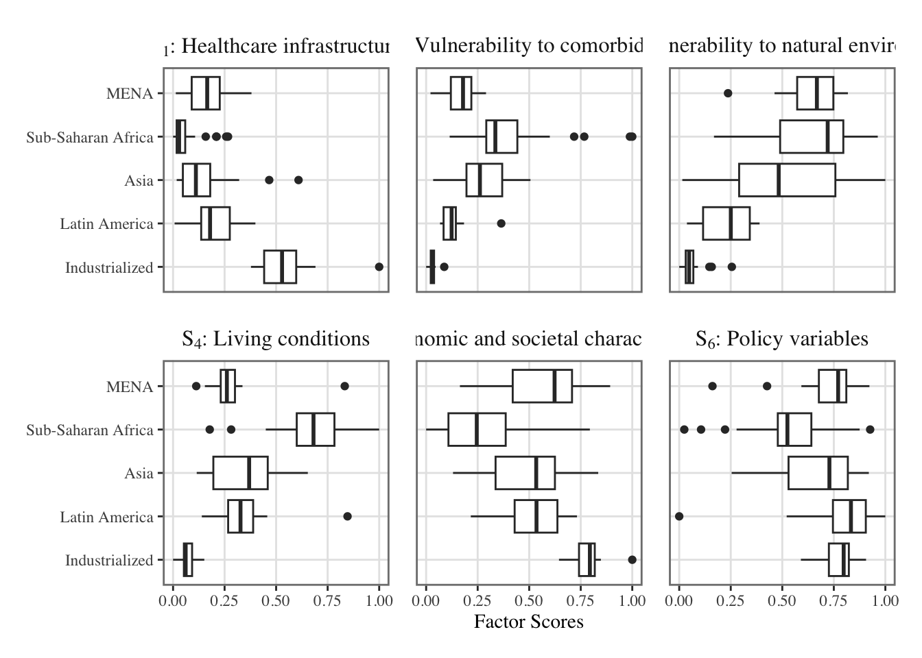
Distribution of factor scores estimated with the Principal Component Analysis in each region.
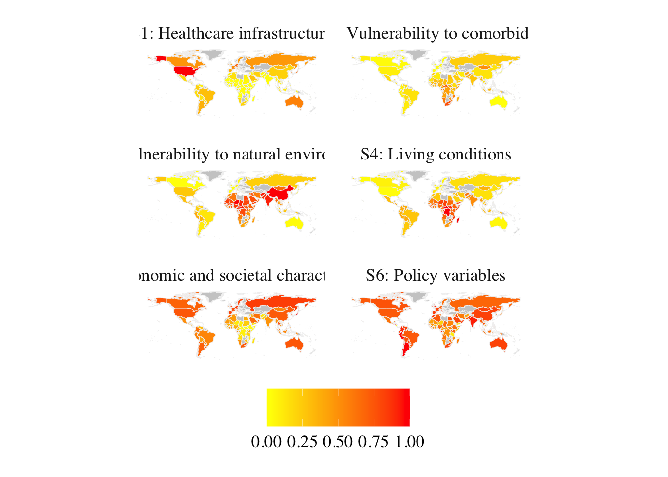
3.5 Maps

Let us define a theme for maps:

#' Theme for maps with ggplot2
#'
#' @param ... arguments passed to the theme function
#' @export
#' @importFrom ggplot2 element_rect element_text element_blank element_line unit
#'   rel
theme_map_paper <- function(...) {
  theme(
    text = element_text(family = "Times"),
    plot.background = element_rect(fill = "transparent", color = NA),
    panel.background = element_rect(fill = "transparent", color = NA),
    panel.border = element_blank(),
    axis.title = element_blank(),
    axis.text = element_blank(),
    axis.ticks = element_blank(), axis.line = element_blank(),
    plot.title.position = "plot",
    legend.text = element_text(size = rel(1.2)),
    legend.title = element_text(size = rel(1.2)),
    legend.background = element_rect(fill="transparent", color = NULL),
    legend.key = element_blank(),
    legend.key.height   = unit(2, "line"),
    legend.key.width    = unit(1.5, "line"),
    strip.background = element_rect(fill = NA),
    panel.spacing = unit(1, "lines"),
    panel.grid.major = element_blank(),
    panel.grid.minor = element_blank(),
    plot.margin = unit(c(1, 1, 1, 1), "lines"),
    strip.text = element_text(size = rel(1.2))
  )
}

A Shapefile that allows us to display the level 0 world administrative boundaries, freely available on the online open data platform “opendatasoft”, can be loaded:

library(sf)
Linking to GEOS 3.11.0, GDAL 3.5.3, PROJ 9.1.0; sf_use_s2() is TRUE
world_map <- sf::read_sf(
  "./data/raw/world-administrative-boundaries/world-administrative-boundaries.shp"
)

There are some mismatching country names between the map file and the epidemic data. The names from the map file can be manually changed:

world_map <- 
  world_map |> 
  mutate(
    name = recode(
      name, 
      # old = new
      "Brunei Darussalam" = "Brunei",
      "Côte d'Ivoire" = "Cote d'Ivoire",
      "Democratic Republic of the Congo" = "Democratic Republic of Congo",
      "Swaziland" = "Eswatini",
      "Iran (Islamic Republic of)" = "Iran",
      "Lao People's Democratic Republic" = "Laos",
      "Russian Federation" = "Russia",
      "Republic of Korea" = "South Korea",
      "Syrian Arab Republic" = "Syria",
      "United Republic of Tanzania" = "Tanzania",
      "U.K. of Great Britain and Northern Ireland" = "United Kingdom",
      "United States of America" = "United States"
    )
  )
df_coordinates_2 <- 
  df_coordinates |> select(country, coord_norm_s1:coord_norm_s6) |> 
  pivot_longer(
    cols = -country,
    names_to = "synthetic_factor",
    values_to = "coord_norm"
  )

world_map_coords <- NULL
# v <- str_c("coord_norm_s", 1:6)[1]
for (v in str_c("coord_norm_s", 1:6)) {
  map_current <- 
    world_map |> 
    left_join(
      df_coordinates_2 |> 
        filter(synthetic_factor == v),
      by = c("name" = "country")
    )
  map_current$synthetic_factor <- v
  
  world_map_coords <- 
    world_map_coords |> bind_rows(map_current)
}

world_map_coords <- 
  world_map_coords |> 
  mutate(
    synthetic_factor = factor(
      synthetic_factor, 
      labels = c("coord_norm_s1" = "S1: Healthcare infrastructure",
                 "coord_norm_s2" = "S2: Vulnerability to comorbidites",
                 "coord_norm_s3" = "S3: Vulnerability to natural environment",
                 "coord_norm_s4" = "S4: Living conditions",
                 "coord_norm_s5" = "S5: Economic and societal characteristics",
                 "coord_norm_s6" = "S6: Policy variables")
    )
  )
p_map <- 
  ggplot(data = world_map_coords) +
  geom_sf(mapping = aes(fill = coord_norm), colour = "gray95", size = .1) +
  scale_fill_gradient(NULL, low = "yellow", high = "red", na.value = "gray80") +
  theme_map_paper() +
  theme(legend.position = "bottom") +
  facet_wrap(~synthetic_factor, ncol = 2)

p_map

Normalised factor scores by countries.