This chapter provides the codes used to obtain the final dataset used in the article. It contains two sections. The first one concerns the Covid-19 epidemic, the second one is devoted to the 2009-2010 H1N1 epidemic.
The {tidyverse} package is needed, as well as {lubridate}:
library(tidyverse)
── Attaching core tidyverse packages ──────────────────────── tidyverse 2.0.0 ──
✔ dplyr     1.1.3     ✔ readr     2.1.4
✔ forcats   1.0.0     ✔ stringr   1.5.0
✔ ggplot2   3.4.4     ✔ tibble    3.2.1
✔ lubridate 1.9.3     ✔ tidyr     1.3.0
✔ purrr     1.0.2
── Conflicts ────────────────────────────────────────── tidyverse_conflicts() ──
✖ dplyr::filter() masks stats::filter()
✖ dplyr::lag()    masks stats::lag()
ℹ Use the conflicted package (<http://conflicted.r-lib.org/>) to force all conflicts to become errors
This section is devoted to Covid-19 data. The first part presents the data relative to the number of cases while the second part shows the socio-economic data associated to each country during the period of the epidemic.
1.1.1 Epidemic Data
The epidemic data come from the COVID-19 Data Repository by the Center for Systems Science and Engineering (CSSE) at Johns Hopkins University (GitHub).
To handle dates properly, some adjustments need to be done:
We can create a table, list_countries, with two columns: one that contains the name of the countries, and another one that gives the group the corresponding country belongs to.
# A tibble: 115 × 2
   country group
   <chr>   <chr>
 1 Algeria MENA
 2 Bahrain MENA
 3 Egypt   MENA
 4 Iran    MENA
 5 Iraq    MENA
 6 Israel  MENA
 7 Jordan  MENA
 8 Kuwait  MENA
 9 Lebanon MENA
10 Morocco MENA
# ℹ 105 more rows
# Run oncedf_oxford <-str_c("https://raw.githubusercontent.com/OxCGRT/covid-policy-tracker/master/data/","OxCGRT_latest.csv") |>read.csv()# Save the raw datasave(df_oxford, file ="./data/raw/df_oxford.rda")
To avoid downloading the data each time we run the program, we can save them and only load the previously downloaded data as follows:
load("./data/raw/df_oxford.rda")
We want to focus only on data at the country level: RegionName must be equal to the empty string.
The cumulative number of cases is contained in value. There are some bizarre values corresponding to statistical adjustments. We can smooth the series of the number of cases using a 7 days rolling windows. To do so, we compute the first difference of the cumulative number of cases to get daily cases, then smooth the data. Lastly, we compute the cumulative number of cases from the smoothed values.
confirmed_df <- confirmed_df |>group_by(country, country_code) |>mutate(c = value -lag(value)) |>mutate(c_7d = zoo::rollmean(c, k =7, fill =NA)) |>mutate(c_7d =ifelse(c_7d <0, yes =0, no = c_7d)) |>group_by(country, country_code) |>mutate(cumul =ifelse(is.na(c_7d), yes =0, no = c_7d),cumul =cumsum(cumul),cumul =ifelse(is.na(value), yes =NA, no = cumul)) |>ungroup()
Then, we replace cumulative number of confirmed cases with the value obtained using a moving average:
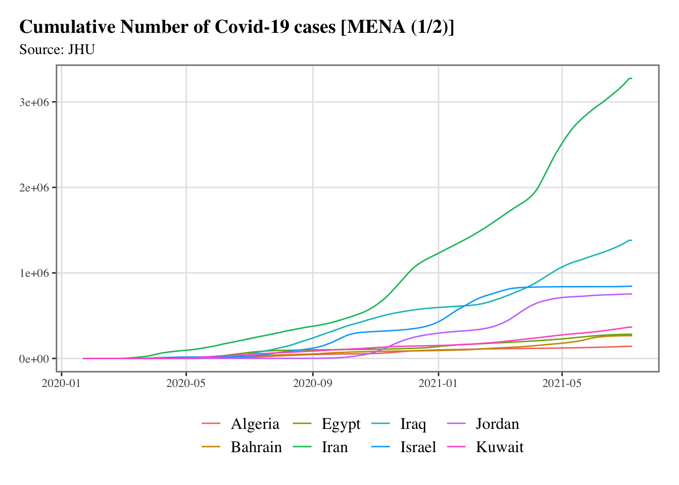
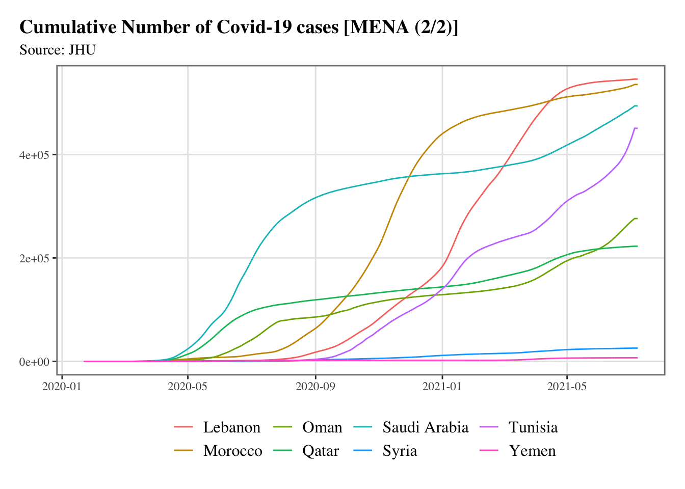
split_chunks <-function(x,n) {split(x, cut(seq_along(x), n, labels =FALSE))}g <-split_chunks(1:length(mena), n =2)for (i in1:length(g)) { p <-ggplot(data = confirmed_df |>filter(country %in% mena[g[[i]]]), mapping =aes(x = date, y = value, colour = country) ) +geom_line() +scale_colour_discrete(NULL) +scale_x_date(breaks =ymd(pretty_dates(confirmed_df$date, n =5)), date_labels ="%Y-%m" ) +labs(x =NULL, y =NULL, title =str_c("Cumulative Number of Covid-19 cases [MENA (", i, "/", length(g), ")]" ),subtitle ="Source: JHU" ) +theme_paper()print(p)}
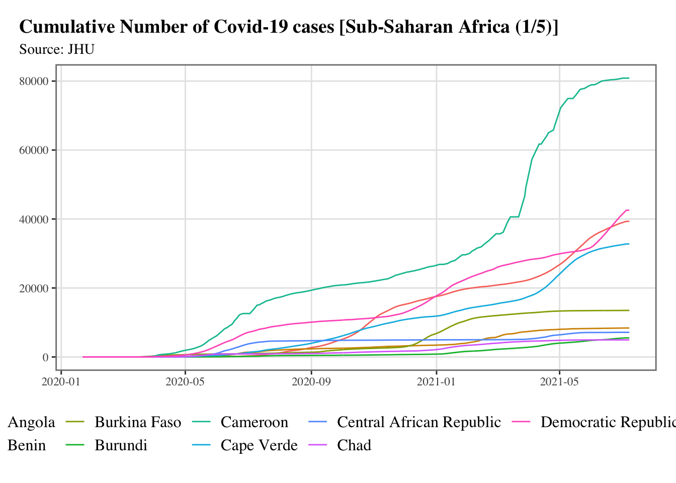
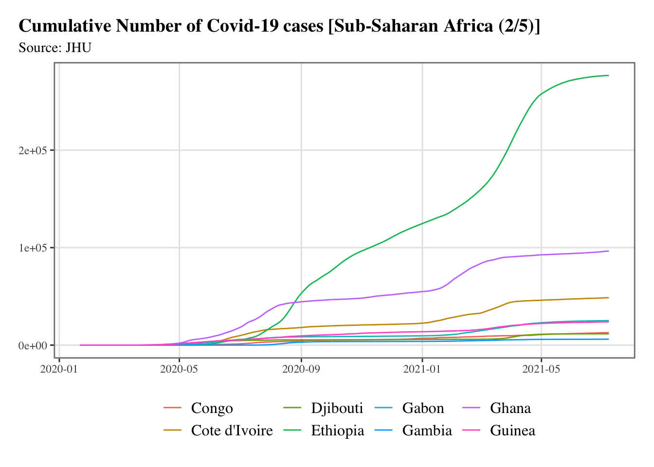
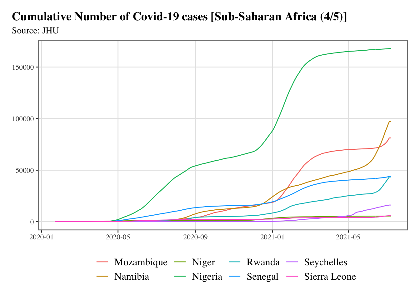
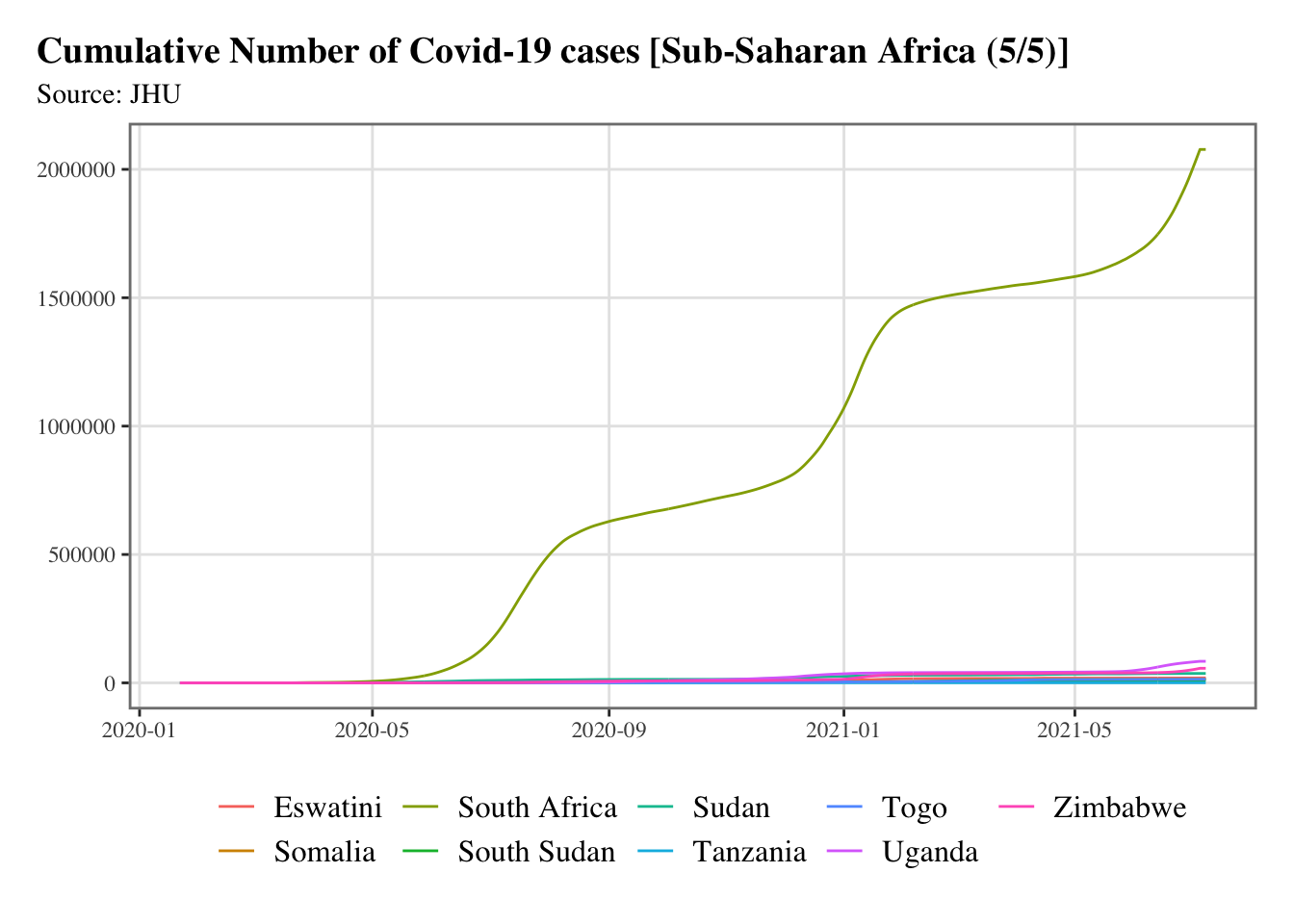
For Sub-Saharan countries:
g <-split_chunks(1:length(ssa), n =5)for (i in1:length(g)) { p <-ggplot(data = confirmed_df |>filter(country %in% ssa[g[[i]]]),mapping =aes(x = date, y = value, colour = country) ) +geom_line() +scale_colour_discrete(NULL) +scale_x_date(breaks =ymd(pretty_dates(confirmed_df$date, n =5)), date_labels ="%Y-%m" ) +labs(x =NULL, y =NULL, title =str_c("Cumulative Number of Covid-19 cases [Sub-Saharan Africa (", i, "/", length(g), ")]" ),subtitle ="Source: JHU") +theme_paper()print(p)}
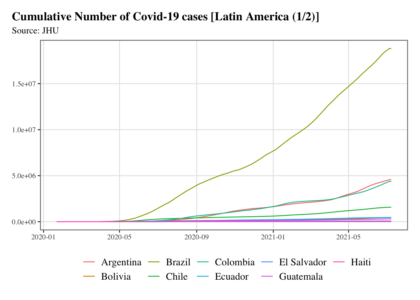
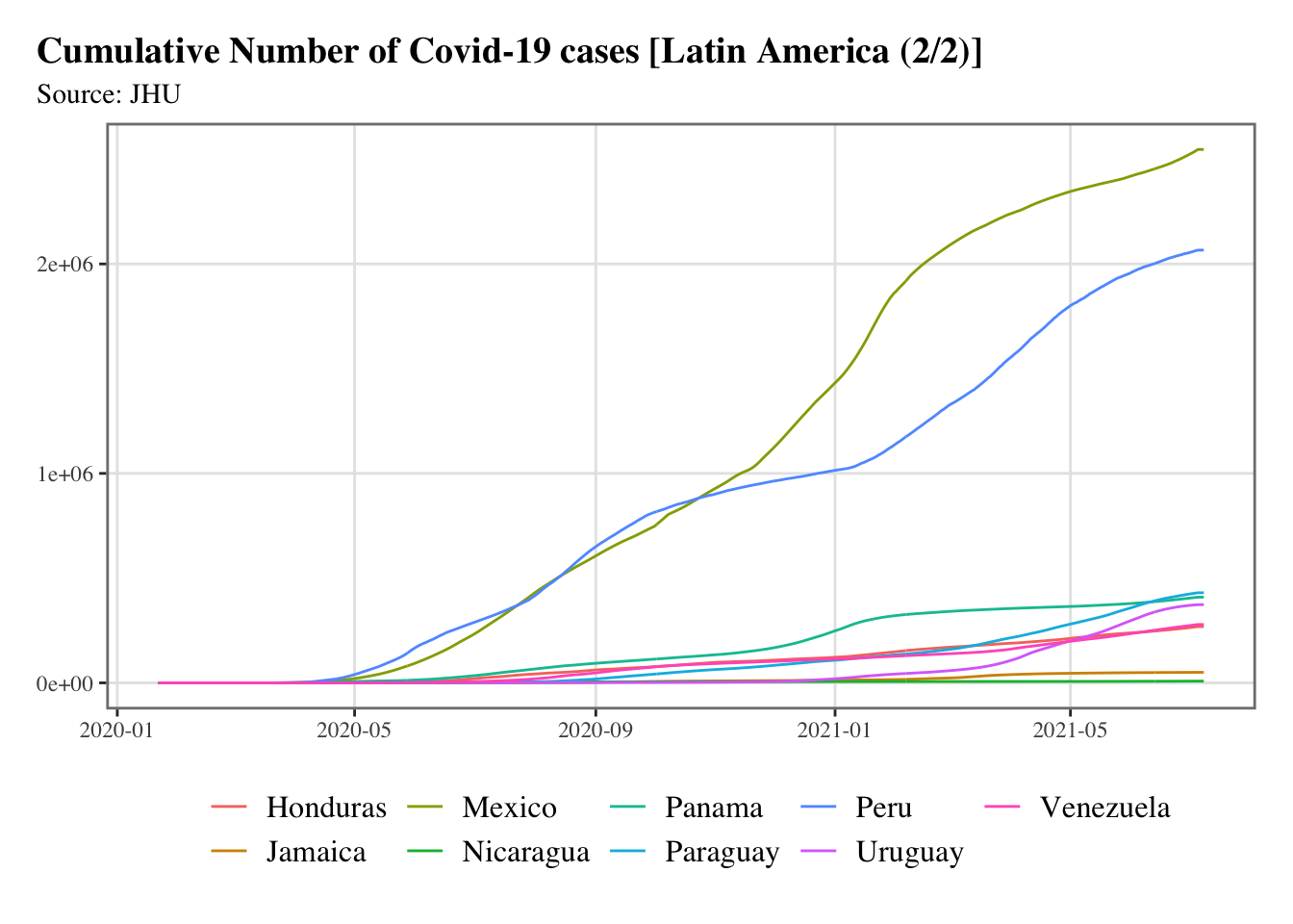
For Latin America:
g <-split_chunks(1:length(latin_america), n =2)for (i in1:length(g)) { p <-ggplot(data = confirmed_df |>filter(country %in% latin_america[g[[i]]]),mapping =aes(x = date, y = value, colour = country) ) +geom_line() +scale_colour_discrete(NULL) +scale_x_date(breaks =ymd(pretty_dates(confirmed_df$date, n =5)), date_labels ="%Y-%m") +labs(x =NULL, y =NULL, title =str_c("Cumulative Number of Covid-19 cases [Latin America (", i, "/", length(g), ")]" ),subtitle ="Source: JHU" ) +theme_paper()print(p)}
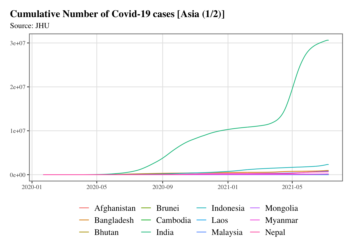
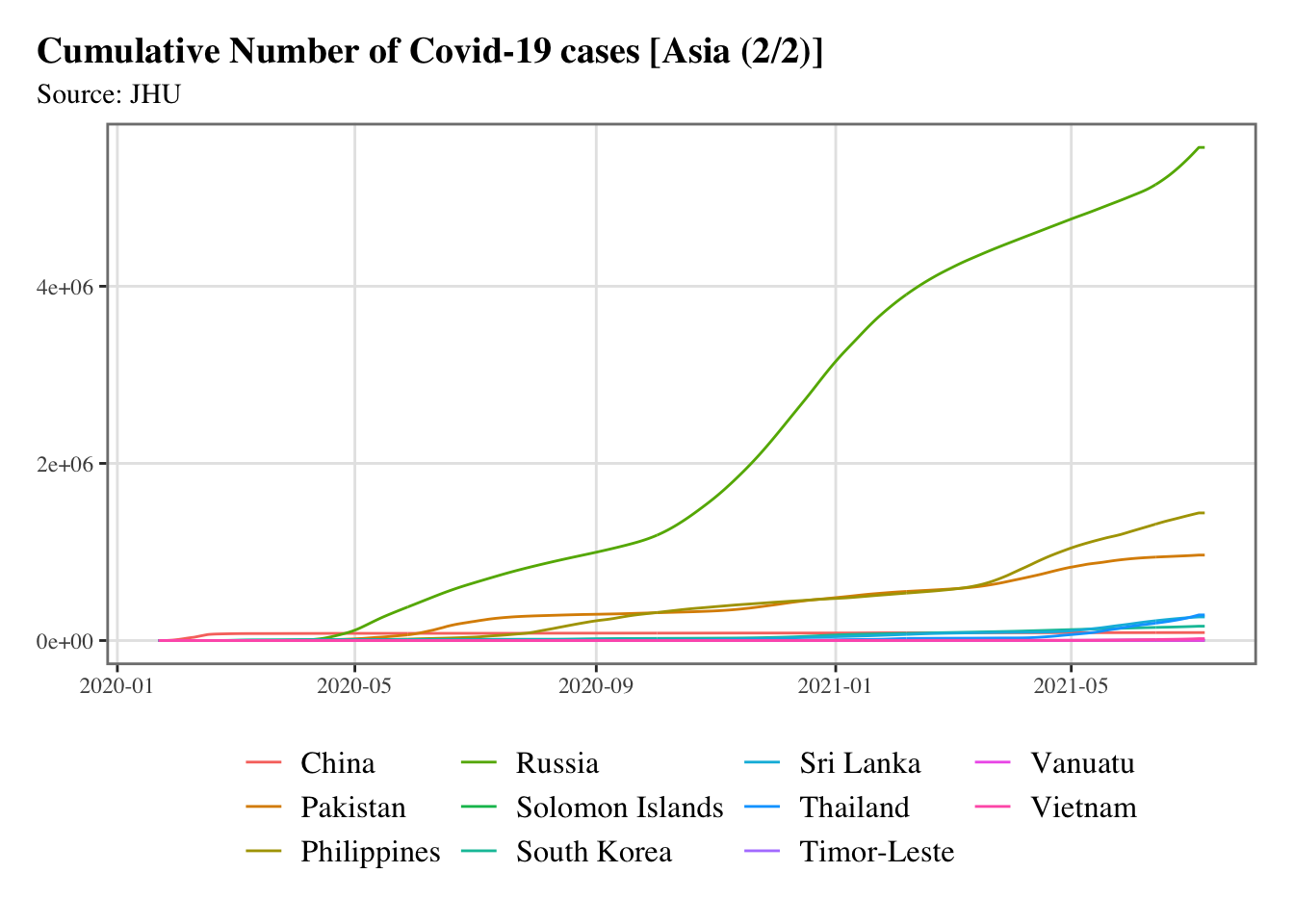
For Asia:
g <-split_chunks(1:length(asia), n =2)for (i in1:length(g)) { p <-ggplot(data = confirmed_df |>filter(country %in% asia[g[[i]]]),mapping =aes(x = date, y = value, colour = country) ) +geom_line() +scale_colour_discrete(NULL) +scale_x_date(breaks =ymd(pretty_dates(confirmed_df$date, n =5)), date_labels ="%Y-%m" ) +labs(x =NULL, y =NULL, title =str_c("Cumulative Number of Covid-19 cases [Asia (", i, "/", length(g), ")]" ),subtitle ="Source: JHU") +theme_paper()print(p)}
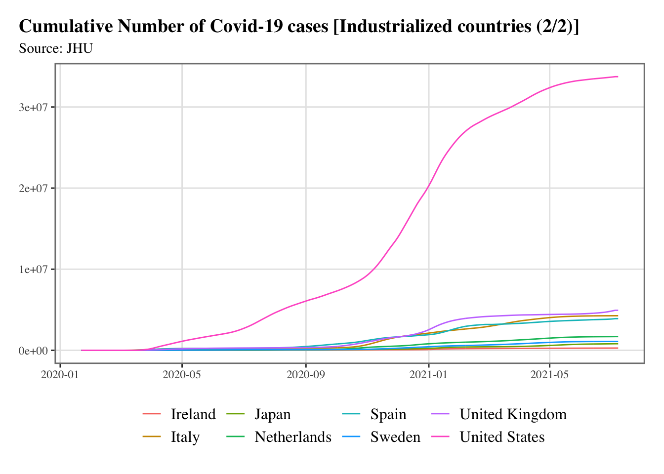
And for industrialized countries:
g <-split_chunks(1:length(indus), n =2)for (i in1:length(g)) { p <-ggplot(data = confirmed_df |>filter(country %in% indus[g[[i]]]),mapping =aes(x = date, y = value, colour = country) ) +geom_line() +scale_colour_discrete(NULL) +scale_x_date(breaks =ymd(pretty_dates(confirmed_df$date, n =5)), date_labels ="%Y-%m" ) +labs(x =NULL, y =NULL, title =str_c("Cumulative Number of Covid-19 cases [Industrialized countries (", i, "/", length(g), ")]" ),subtitle ="Source: JHU" ) +theme_paper()print(p)}
The variables that are kept in the study are divided in 6 categories, 5 of which that concern the WDI database. The 6th (Policy variables and governance) is extracted from the Oxford COVID-19Government Response Tracker.
# S1: Healthcare infrastructurevariables_to_keep_S1 <-c("Physicians (per 1,000 people)","Hospital beds (per 1,000 people)","Nurses and midwives (per 1,000 people)","Domestic general government health expenditure (% of general government expenditure)","Domestic private health expenditure per capita (current US$)","Domestic private health expenditure per capita, PPP (current international $)")# S2: Vulnerability to comorbiditiesvariables_to_keep_S2 <-c("Incidence of malaria (per 1,000 population at risk)","Incidence of HIV, all (per 1,000 uninfected population)","Incidence of tuberculosis (per 100,000 people)","Diabetes prevalence (% of population ages 20 to 79)","Mortality from CVD, cancer, diabetes or CRD between exact ages 30 and 70 (%)")# S3: Vulnerability to natural environmentvariables_to_keep_S3 <-c("Mortality rate attributed to household and ambient air pollution, age-standardized (per 100,000 population)","PM2.5 air pollution, mean annual exposure (micrograms per cubic meter)","PM2.5 pollution, population exposed to levels exceeding WHO Interim Target-1 value (% of total)","PM2.5 pollution, population exposed to levels exceeding WHO Interim Target-2 value (% of total)","PM2.5 pollution, population exposed to levels exceeding WHO Interim Target-3 value (% of total)","Air transport, passengers carried","International tourism, number of arrivals","Ecological Footprint")# S4: Living conditionsvariables_to_keep_S4 <-c(# "Multidimensional poverty index (scale 0-1)",# No data..."People using at least basic drinking water services (% of population)","People using at least basic sanitation services (% of population)","Prevalence of undernourishment (% of population)","Prevalence of anemia among women of reproductive age (% of women ages 15-49)","Poverty headcount ratio at $3.65 a day (2017 PPP) (% of population)","Poverty headcount ratio at $6.85 a day (2017 PPP) (% of population)","Poverty headcount ratio at national poverty lines (% of population)","GDP per capita (current US$)","GDP per capita, PPP (current international $)","Urban population", # Will not be kept in PCA"Urban land area (sq. km)", # Will not be kept in PCA"Urban density")#S5: Economic and societal characteristicsvariables_to_keep_S5 <-c("Population, total","GDP per capita growth (annual %)","International migrant stock (% of population)","Population ages 65 and above (% of total population)","Individuals using the Internet (% of population)","Mobile cellular subscriptions (per 100 people)","Gini index (World Bank estimate)", # Will no be kept in PCA"Gini index (CIA estimate)","Shadow size Economy")# c("Shadow size Economy", "Ecological Footprint", "Gini index (CIA estimate)")#S6: Policy variables and governancevariables_to_keep_S6 <-c("GovernmentResponseIndex","ContainmentHealthIndex", "StringencyIndex","EconomicSupportIndex")variables_to_keep <-c( variables_to_keep_S1, variables_to_keep_S2, variables_to_keep_S3, variables_to_keep_S4, variables_to_keep_S5, variables_to_keep_S6)
For convenience, a table that contains the list of variable and their type can be created:
variables_to_keep_df <-tibble(variable = variables_to_keep_S1, type ="S1") |>bind_rows(tibble(variable = variables_to_keep_S2, type ="S2")) |>bind_rows(tibble(variable = variables_to_keep_S3, type ="S3")) |>bind_rows(tibble(variable = variables_to_keep_S4, type ="S4")) |>bind_rows(tibble(variable = variables_to_keep_S5, type ="S5")) |>bind_rows(tibble(variable = variables_to_keep_S6, type ="S6"))variables_to_keep_df
# A tibble: 44 × 2
   variable                                                                type
   <chr>                                                                   <chr>
 1 Physicians (per 1,000 people)                                           S1
 2 Hospital beds (per 1,000 people)                                        S1
 3 Nurses and midwives (per 1,000 people)                                  S1
 4 Domestic general government health expenditure (% of general governmen… S1
 5 Domestic private health expenditure per capita (current US$)            S1
 6 Domestic private health expenditure per capita, PPP (current internati… S1
 7 Incidence of malaria (per 1,000 population at risk)                     S2
 8 Incidence of HIV, all (per 1,000 uninfected population)                 S2
 9 Incidence of tuberculosis (per 100,000 people)                          S2
10 Diabetes prevalence (% of population ages 20 to 79)                     S2
# ℹ 34 more rows
1.1.2.2 WDI data
The study relies on socio-economic data. Most variables are extracted from the World Development Indicators (WDI) from the World Bank.
We downloaded a bulk CSV file version of the database. The data can then easily be loaded into R:
wdi_df <-read_csv("./data/raw/WDI_csv.zip")
Multiple files in zip: reading 'WDIData.csv'
New names:
Rows: 392882 Columns: 68
── Column specification ────────────────────────────────────────────────────────
Delimiter: ","
chr  (4): Country Name, Country Code, Indicator Name, Indicator Code
dbl (63): 1960, 1961, 1962, 1963, 1964, 1965, 1966, 1967, 1968, 1969, 1970, ...
lgl  (1): ...68

ℹ Use `spec()` to retrieve the full column specification for this data.
ℹ Specify the column types or set `show_col_types = FALSE` to quiet this message.
Since the last column contains only NA values, it should be removed:
[1] "Access to clean fuels and technologies for cooking (% of population)"
[2] "Access to clean fuels and technologies for cooking, rural (% of rural population)"
[3] "Access to clean fuels and technologies for cooking, urban (% of urban population)"
[4] "Access to electricity (% of population)"
[5] "Access to electricity, rural (% of rural population)"
[6] "Access to electricity, urban (% of urban population)"
We have selected a few variables from the database. To be able to correctly identify the names of the variables we are interested in, we used the following piece of code (here is an example to identify variables that contain the word ‘poverty’):
Let us rename some countries in the WDI dataset so that their names match those that can be found in the Oxford dataset.
wdi_df <- wdi_df |>mutate(`Country Name`=recode(`Country Name`,# old = new"Brunei Darussalam"="Brunei","Cabo Verde"="Cape Verde","Congo, Dem. Rep."="Democratic Republic of Congo","Congo, Rep."="Congo","Egypt, Arab Rep."="Egypt","Gambia, The"="Gambia","Hong Kong SAR, China"="Hong Kong","Iran, Islamic Rep."="Iran","Korea, Rep."="South Korea","Lao PDR"="Laos","Russian Federation"="Russia","Syrian Arab Republic"="Syria","Venezuela, RB"="Venezuela","Yemen, Rep."="Yemen" ) )
1.1.2.3 Ecological Footprint
We extract the ecological footprint data from the Global Footprint Network National Footprint and Biocapacity Accounts. It measures, in gobal hectares, ‘how much area of biologically productive land and water an individual, population, or activity requires to produce all the resources it consumes and to absorb the waste it generates, using prevailing technology and resource management practices.’
To get the data, we made some queries to the API, after creating an account (for free). This notebook will present the way to get the data, but to avoid making unecessary requests to the API, the data are loaded from a previous call to the API.
library(rvest)library(httr)
The username and API key need to be sent at each call.
We created a simple function, as explained in the R vignette of {httr}, to make a call to the API:
#' Request made to footprintnetwork.org API#' #' @param url endpoint#' url <- "http://api.footprintnetwork.org/v1/types"request_api <-function(url) { resp <-GET(url, authenticate(username, key))if (http_type(resp) !="application/json") {stop("API did not return json", call. =FALSE) } jsonlite::fromJSON(content(resp, "text"), simplifyVector =TRUE)}# End of request_api()
We defined a function that prepares the URL depending on the country code, the year and the type of data:
#' Fetch data from footprintnetwork.org API#' @param country_code code of the country (e.g., 68 for France, or all for all countries)#' @param year year#' @param data_type Record type taken from types list or 'all' (e.g., pop)get_data_country <-function(country_code, year, data_type) { url <-str_c("http://api.footprintnetwork.org/v1/data/", country_code, "/", year, "/", data_type )request_api(url)}
Then, we make a simple call to the API to list of variables that can be asked:
We rely on the estimates of the size of the Shadow Economy reported in Medina and Schneider (2019). The data reported in table A.1 from the Appendix of their paper have been manually extracted and saved in a CSV file.
ℹ Using "','" as decimal and "'.'" as grouping mark. Use `read_delim()` for more control.
Rows: 157 Columns: 2
── Column specification ────────────────────────────────────────────────────────
Delimiter: ";"
chr (1): ISO
num (1): shadow_size

ℹ Use `spec()` to retrieve the full column specification for this data.
ℹ Specify the column types or set `show_col_types = FALSE` to quiet this message.
Rows: 173 Columns: 6
── Column specification ────────────────────────────────────────────────────────
Delimiter: ","
chr (4): name, slug, date_of_information, region
dbl (2): value, ranking

ℹ Use `spec()` to retrieve the full column specification for this data.
ℹ Specify the column types or set `show_col_types = FALSE` to quiet this message.
Some countries need to be renamed to match those of the Oxford dataset:
We filter the data to keep the period from January 2020 to January 2021 and compute an average of the variables of interes (variables_to_keep_S6) over the period:
Warning: Using an external vector in selections was deprecated in tidyselect 1.1.0.
ℹ Please use `all_of()` or `any_of()` instead.
  # Was:
  data %>% select(variables_to_keep_S6)

  # Now:
  data %>% select(all_of(variables_to_keep_S6))

See <https://tidyselect.r-lib.org/reference/faq-external-vector.html>.
`summarise()` has grouped output by 'country'. You can override using the
`.groups` argument.
We create a function that allows us to create and export a database for each group of countries. This database contains the 2020 value for each variable. When the 2020 value was missing in the data, we took the average value over the last 5 years. For the remaining missing values, we took the 10 years average, or the 15 years average. When there was no data available in the selected years, we replaced the missing value by the average of the region.
#'@param countries group of countries#'@param file export databaseget_out_countries <-function(countries, file) { df_countries_wdi <- wdi_df |># Keeping countries of interestfilter(`Country Name`%in%!!countries) |># And variables of interestfilter(`Indicator Name`%in%!!variables_to_keep) |>pivot_longer(cols =`1960`:`2020`, names_to ="year") |>select(ISO =`Country Code`, country =`Country Name`, variable =`Indicator Name`, year, value) df_countries_wdi <- df_countries_wdi |>mutate(year =as.numeric(year)) |>filter(year >=2005) |>mutate(value_2020 =ifelse(year ==2020, yes = value, no =NA),value_last_5 =ifelse(year %in%seq(2015,2020), yes = value, no =NA),value_last_10 =ifelse(year %in%seq(2010,2020), yes = value, no =NA),value_last_15 =ifelse(year %in%seq(2005,2020), yes = value, no =NA) ) |>pivot_longer(cols = value_2020:value_last_15, names_to ="var", values_to ="replacement_val" ) |>group_by(ISO, country, variable, var) |>summarise(# nb_val = sum(!is.na(replacement_val)),replacement_val =mean(replacement_val, na.rm =TRUE) ) |>pivot_wider(names_from = var, values_from = replacement_val) |>mutate(# If missing value: average of the 5 previous yearstype =ifelse(is.na(value_2020) |is.nan(value_2020), yes ="last 5", no ="value 2020" ),value =ifelse(is.na(value_2020) |is.nan(value_2020), yes = value_last_5, no = value_2020 ) ) |>mutate(# If missing value: average of the 10 previous yearstype =ifelse(is.na(value) |is.nan(value), yes ="last 10", no = type ),value =ifelse(is.na(value) |is.nan(value), yes = value_last_10, no = value ) ) |>mutate(# If missing value: average of the 15 previous yearstype =ifelse(is.na(value) |is.nan(value), yes ="last 15", no = type ),value =ifelse(is.na(value) |is.nan(value), yes = value_last_15, no = value ) ) |>mutate(# If missing value: NAtype =ifelse(is.na(value) |is.nan(value), yes ="flag", no = type),value =ifelse(is.na(value) |is.nan(value), yes =NA, no = value) ) |>select(-value_2020, -value_last_5, -value_last_10, -value_last_15)# Malaria set to 0 when it is NA, in 2020 df_countries_wdi <- df_countries_wdi |>mutate(value =ifelse( variable =="Incidence of malaria (per 1,000 population at risk)"&is.na(value),yes =0, no = value) )# Ecological Footprint df_countries_footprint <-# corresp_iso |> # filter(country %in% countries) |> # left_join(df_footprint, by = c("ISO", "country")) |> df_footprint |>filter(country %in%!!countries) |>mutate(variable ="Ecological Footprint") |>mutate(type =str_c(year, " est.")) |>select(-year, -countryName)# Gini df_countries_gini <-# corresp_iso |> # filter(country %in% countries) |> # left_join(df_cia, by = c("ISO", "country")) |> df_cia |>filter(country %in%!!countries) |>rename(type = date_of_information) |>select(country, value, type) |>mutate(variable ="Gini index (CIA estimate)")# Shadow Size of the epidemic df_shadow_size <- confirmed_df |>select(country, country_code) |>unique() |>filter(country %in% countries) |>left_join( df_shadow_economy, by =c("country_code"="ISO") ) |>rename(value = shadow_size) |>mutate(variable ="Shadow size Economy",type ="2015 est." ) |>select(country, value, type, variable) df_countries <- df_countries_wdi |>ungroup() |>select(-ISO) |>bind_rows(df_countries_footprint) |>bind_rows(df_countries_gini) |>bind_rows(df_shadow_size) |>ungroup() df_countries <- df_countries |>complete(country, variable) df_countries <- df_countries |>mutate(type =ifelse(is.na(type), yes ="flag", no = type))# Average within the zone group_average <- df_countries |>group_by(variable) |>summarise(value_group =mean(value, na.rm=TRUE))# Replacing missing values with group average df_countries <- df_countries |>left_join(group_average, by ="variable") |>mutate(# If missing value: group averagetype =ifelse(is.na(value) |is.nan(value), yes ="group average", no = type ),value =ifelse(is.na(value) |is.nan(value), yes = value_group, no = value ) ) |>select(-value_group)# Variables in columns df_countries <- df_countries |>pivot_wider(names_from = variable, values_from =c(type, value))# select(# ISO, country, str_c(c("value_", "type_"), rep(variables_to_keep, each = 2))# ) df_countries <- df_countries |># Computing Urban densitymutate(`value_Urban density`=`value_Urban population`/`value_Urban land area (sq. km)`,`type_Urban density`=`type_Urban population`)# Adding Oxford indicators df_countries_excel <- df_countries |>left_join(df_oxford_year, by ="country")# Table with summary of missing data df_missing <- df_countries_excel |>select(country, starts_with("type_")) |>pivot_longer(cols =-c(country), names_to ="variable") |>group_by(variable, value) |>summarise(n =n()) |>group_by(variable) |>mutate(freq = scales::percent(n /sum(n), accuracy =0.1)) |>select(-n) |>pivot_wider(names_from = value, values_from = freq, values_fill ="") |>mutate(variable =str_remove(variable, "^type_"),variable =factor(variable, levels = variables_to_keep)) |>arrange(variable)# reordering the columns vn <-c("variable", "2020", "last 5", "last 10", "last 15", "group average") vn <- vn[vn %in%colnames(df_missing)] vn2 <-sort(colnames(df_missing)[!colnames(df_missing)%in%vn]) df_missing <- df_missing |>select(!!vn, !!vn2) write_excel_csv(df_countries_excel, file = file)list(df_countries_excel = df_countries_excel, df_missing = df_missing)} # End of get_out_countries()
`summarise()` has grouped output by 'ISO', 'country', 'variable'. You can
override using the `.groups` argument.
`summarise()` has grouped output by 'variable'. You can override using the
`.groups` argument.
`summarise()` has grouped output by 'ISO', 'country', 'variable'. You can
override using the `.groups` argument.
`summarise()` has grouped output by 'variable'. You can override using the
`.groups` argument.
`summarise()` has grouped output by 'ISO', 'country', 'variable'. You can
override using the `.groups` argument.
`summarise()` has grouped output by 'variable'. You can override using the
`.groups` argument.
`summarise()` has grouped output by 'ISO', 'country', 'variable'. You can
override using the `.groups` argument.
`summarise()` has grouped output by 'variable'. You can override using the
`.groups` argument.
`summarise()` has grouped output by 'ISO', 'country', 'variable'. You can
override using the `.groups` argument.
`summarise()` has grouped output by 'variable'. You can override using the
`.groups` argument.
if (knitr::is_html_output()) { population |> DT::datatable(options =list(searching =TRUE,pageLength =10,lengthMenu =c(5, 10, 15, 20) )) }
1.3 Summary
File
Description
Source
./data/output/covid_cases.rda
Daily cumulative number of Covid-19 cases
JHU
./data/output/covid/df_all_countries.csv
Socio-Economic variables for countries for the Covid-19 period
World Development Indicators, Global Footprint Network National Footprint and Biocapacity Accounts, Medina and Schneider (2019), CIA, Hale et al. (2021)
./data/output/population.rda
Population
World Development Indicators
Hale, Thomas, Noam Angrist, Rafael Goldszmidt, Beatriz Kira, Anna Petherick, Toby Phillips, Samuel Webster, et al. 2021. “A Global Panel Database of Pandemic Policies (Oxford COVID-19 Government Response Tracker).”Nature Human Behaviour. https://doi.org/10.1038/s41562-021-01079-8.
Medina, Leandro, and Friedrich Schneider. 2019. “Shedding Light on the Shadow Economy: A Global Database and the Interaction with the Official One.”