2  Word colouring on graphs

I sometimes want some words to appear in a specific color on plots made with ggplot2.

library(tidyverse)

── Attaching core tidyverse packages ──────────────────────── tidyverse 2.0.0 ──
✔ dplyr     1.1.3     ✔ readr     2.1.4
✔ forcats   1.0.0     ✔ stringr   1.5.0
✔ ggplot2   3.4.4     ✔ tibble    3.2.1
✔ lubridate 1.9.3     ✔ tidyr     1.3.0
✔ purrr     1.0.2     
── Conflicts ────────────────────────────────────────── tidyverse_conflicts() ──
✖ dplyr::filter() masks stats::filter()
✖ dplyr::lag()    masks stats::lag()
ℹ Use the conflicted package (<http://conflicted.r-lib.org/>) to force all conflicts to become errors

library(ggtext)

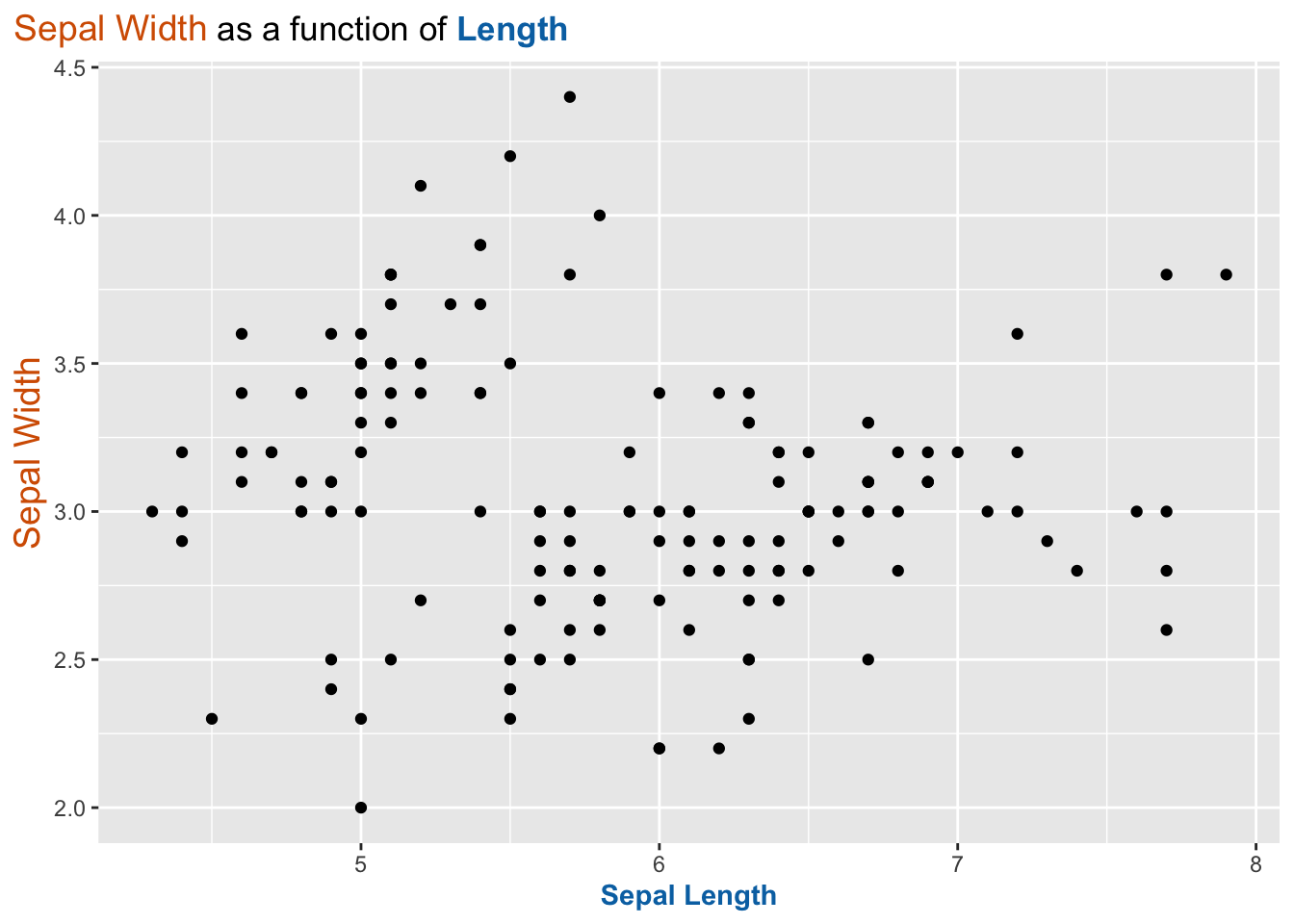
2.1 Title and axis

We use the span HTML element to put hexadecimal colors we desire for some text in the arguments x, y or title of the labs() function. Then, we need to update theme() function so that the elements axis.title.x, axis.title.y, and plot.title are correctly interpreted.

ggplot(
  data = iris,
  mapping = aes(
    x = Sepal.Length,
    y = Sepal.Width
  )
) +
  geom_point() +
  labs(
    x = "<span style='color:#0072B2;'>**Sepal Length**</span>",
    y = "<span style='font-size:14pt; color:#D55E00;'>Sepal Width</span>",
    title = str_c("<span style='font-size:14pt; color:#D55E00;'>Sepal Width",
                  "</span> as a function of <span style='color:#0072B2;'>",
                  "**Length**</span>")
  ) + 
  theme(
    plot.title.position = "plot",
    axis.title.x = element_markdown(),
    axis.title.y = element_markdown(),
    plot.title = element_markdown()
  )

2.2 Facets

First, we define the colours.

col_species <- tribble(
  ~Species, ~colours_species,
  "setosa", "#1b9e77",
  "versicolor",  "#d95f02",
  "virginica", "#7570b3"
)

Then, using {glue}, we put the facet text in a span element, with the associated colour.

library(glue)
library(ggtext)
df_plot <- 
  iris %>% 
  left_join(col_species, by = "Species") %>% 
  mutate(
    type = glue(
      "<span style='color:{colours_species};'>{Species}</span>"
    ),
    type = as.character(type)
  )

df_plot$type[1]

[1] "<span style='color:#1b9e77;'>setosa</span>"

Then, using {ggtext} element_markdown() function, the text can be interpreted as markdown.

ggplot(
  data = df_plot,
  mapping = aes(
    x = Sepal.Length,
    y = Sepal.Width
  )
) +
  geom_point() +
  facet_wrap(~type) +
  theme(
    strip.text = element_markdown(),
    strip.text.x = element_markdown(),
    strip.text.y = element_markdown()
  )

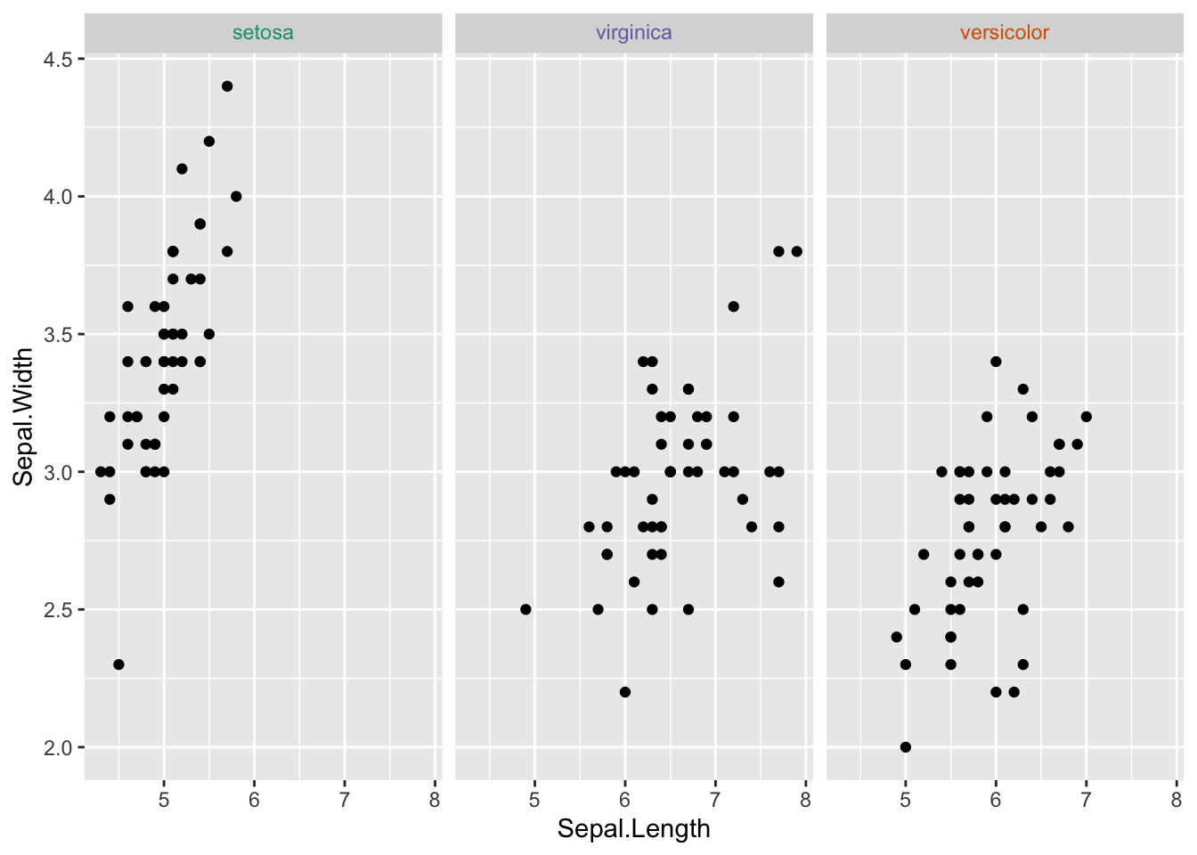
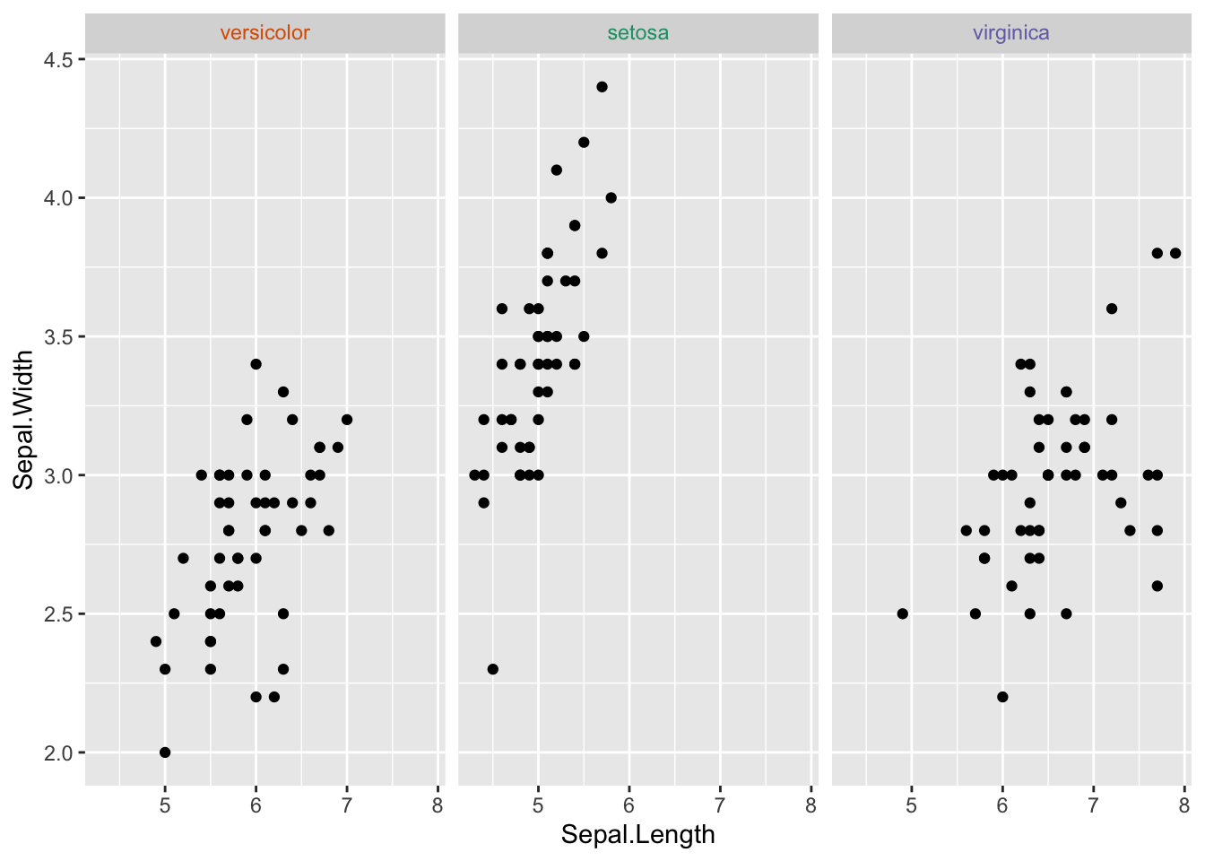
2.2.1 With a different order for the facet elements

We can use a trick, using {forcats} fct_reorder() function:

1. In a first step, we relevel the orginial variables that is used to create the faceting groups (not the one we just created to make it as a markdown string), using factor(), for example.
2. In a second step, we use the fct_reorder() on the variable used to create the faceting groups (the one we just created as a markdown string) and we apply the order of the numerical values corresponding to the levels of the releveled variables from Step 1.

df_plot <- 
  df_plot %>% 
  mutate(
    Species = factor(
      Species, levels = c("versicolor", "setosa", "virginica")),
    type = fct_reorder(type, as.numeric(Species))
  )

ggplot(
  data = df_plot,
  mapping = aes(
    x = Sepal.Length,
    y = Sepal.Width
  )
) +
  geom_point() +
  facet_wrap(~type) +
  theme(
    strip.text = element_markdown(),
    strip.text.x = element_markdown(),
    strip.text.y = element_markdown()
  )

Keywords: ggplot2 markdown color colour