Data Visualization with R

Chapter 2 – Data Wrangling with {dplyr} and {tidyr}

Ewen Gallic

September 2, 2026

Disclaimers

The content of this presentation was adapted from the teaching material provided by Ségal Le Guern Herry who kindly shared his slide deck.
I used Gemini 3.6 Flash to help producing the slides (assistance in organizing content and producing clearer sentences).

Tidying Data

What is `dplyr`?

dplyr is a grammar of data manipulation. It provides a clean, consistent set of “verbs” for common data wrangling tasks.
It is part of a core ecosystem called tidyverse (you are encouraged to read the tidyverse style guide for clean code formatting).
Why should you use dplyr?
- It is highly readable, expressive, and optimized for data manipulation workflows.

Handling Ultra-High-Dimensional with R

For ultra-high-dimensional datasets with tens of thousands of columns or gigabytes of memory overhead, high-performance packages like {data.table} offer an alternative approach.

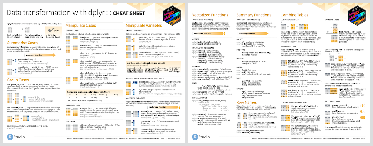
Cheat Sheet

If you are willing to decorate your room, do not hesitate to print this awesome cheat sheet.

Core Syntax of `dplyr`

The functions in {dplyr} are designed for tabular data, they are built specifically to manipulate data.frame and tibble objects (more modern tables).
Every action is defined by a descriptive function, named a verb.
- Example: mutate() creates, modifies, or deletes columns.
{dplyr} adopts a consistent function syntax:

\[ \text{verb}(\underbrace{.data}_{\text{1st argument}},\, \underbrace{other\, arguments}_{\text{2nd to } n\text{-th arguments}}) \]

Key Property of dplyr Verbs

The first argument is always a data frame, and the function always returns a new data frame. This structure makes chaining with pipes (|>) intuitive (see next slide).

The Pipe Operator (`|>` or `%>%`)

The pipe operator passes the output of the left side as the first argument to the function on the right side.

\[ \text{data} \;\mathbf{|>}\; \text{verb}_1(\dots) \;\mathbf{|>}\; \text{verb}_2(\dots) \]

The Data Refining Pipeline

flowchart LR
    A["<b>Crude Oil</b><br/><br/>Raw Dataset"]
    B["<b>Refinery Station 1</b><br/><br/><code>filter(...)</code>"]
    X["<b>More stations...</b><br/><br/><code>verb(...)</code>"]
    C["<b>Refinery Station N</b><br/><br/><code>mutate(...)</code>"]
    D["<b>Premium Fuel</b><br/><br/>Clean Data"]

    A -->|"|>"| B
    B -->|"|>"| X
    X -->|"|>"| C
    C -->|"|>"| D

    style A fill:#ffe5cc,stroke:#cc6600
    style B fill:#e6f0ff,stroke:#3366cc
    style X fill:#f5f5f5,stroke:#888888,stroke-dasharray: 5 5
    style C fill:#e6f0ff,stroke:#3366cc
    style D fill:#e5f5e5,stroke:#339933

Why Using The Data Refining Pipeline?

Nested Syntax (Hard to Read):

# Evaluated inside-out!
summarise(
  group_by(
    filter(law, UGPA > 3.0),
    race
  ),
  mean_lsat = mean(LSAT)
)

Piped Syntax (Reads Left-to-Right):

# Clean, sequential data flow!
law |>
  filter(UGPA > 3.0) |>
  group_by(race) |>
  summarise(mean_lsat = mean(LSAT))

Native Pipe vs. Magrittr

Use the native R pipe |> (R \(\ge\) 4.1.0). In older code bases, you may also see the {magrittr} pipe %>%.

Loading the Law School Dataset

To illustrate {dplyr} verbs, we load the law school dataset (Wightman 1998) using read_csv() from {readr}. This reads the .csv file into a tibble (the tidyverse version of a data frame):

library(readr) ; library(here)
law <- read_csv(file = here("data", "law_data.csv"))
law

# A tibble: 21,791 × 9
    ...1 race       sex  LSAT  UGPA region_first  ZFYA sander_index first_pf
   <dbl> <chr>    <dbl> <dbl> <dbl> <chr>        <dbl>        <dbl>    <dbl>
 1     0 White        1  39     3.1 GL           -0.98        0.783        1
 2     1 White        1  36     3   GL            0.09        0.736        1
 3     2 White        2  30     3.1 MS           -0.35        0.670        1
 4     5 Hispanic     2  39     2.2 NE            0.58        0.697        1
 5     6 White        1  37     3.4 GL           -1.26        0.786        1
 6     7 White        1  30.5   3.6 GL            0.3         0.724        1
 7     8 White        2  36     3.6 GL           -0.1         0.793        1
 8     9 White        2  37     2.7 NE           -0.12        0.720        0
 9    13 White        1  37     2.6 GL            1.53        0.710        1
10    14 White        2  31     3.6 GL            0.34        0.730        1
# ℹ 21,781 more rows

⚙️ Reproducible File Paths with `{here}`

Hardcoding file paths or using setwd() breaks code when sharing projects across different operating systems and nested folder structures. The {here} package provides robust, platform-independent paths.

Fragile Approaches

Hardcoded Absolute Paths:

# Fails on macOS/Linux and other machines!
read_csv("C:/Users/ewen/project/data/law_data.csv")

Manual setwd():

# Breaks Quarto rendering and script portability
setwd("data/")

Note that path separators are different depending on the OS: * Windows uses backslashes (\), * macOS/Linux use forward slashes (/)

The `here()` Solution

# Builds: [Project Root]/data/law_data.csv
read_csv(here("data", "law_data.csv"))

Locates Project Root: Scans upwards to locate the .Rproj file or .git directory, making paths relative to the project root.
OS-Agnostic Concatenation: Combines directory arguments using the host OS’s native separator (/ vs \).

Dataset Overview & Variables

The dataset contains individual-level data on law school students across the United States:

Variable	Type	Description
`...1`	numeric	Row identifier / index
`race`	character	Self-reported race (Amerindian, Asian, Black, Hispanic, Mexican, Other, Puertorican, White)
`sex`	numeric	Sex of the student (`1` = Female, `2` = Male)
`LSAT`	numeric	LSAT score received by the student (measured on a 10 to 48 scale)
`UGPA`	numeric	Undergraduate GPA of the student (from 0 to 4.33)
`region_first`	character	Geographic region where the student took their first bar examination (Far West, Great Lakes, Midsouth, Midwest, Mountain West, Northeast, New England, Northwest, South Central, South East)
`ZFYA`	numeric	Standardized First-Year Average law school grades (FYA)
`sander_index`	numeric	Composite index weighting LSAT and UGPA (\(200 \times \text{UGPA} + \text{LSAT}\))
`first_pf`	numeric	Binary indicator for passing the bar exam on the first trial (`1` = Pass, `0` = Fail)

Core `dplyr` Verbs Overview

Data wrangling in {dplyr} relies on a set of core “verbs” designed to manipulate tabular data:

Verb	Action	Typical Use Case
`filter()`	Subset rows	Keep observations matching specific logical criteria
`arrange()`	Reorder rows	Sort data in ascending or descending order
`select()`	Subset columns	Keep, drop, or rename specific variables
`mutate()`	Create / modify columns	Compute new variables or alter existing ones
`summarise()`	Aggregate data	Collapse multiple rows into group summary metrics
`group_by()`	Group observations	Structure operations to execute per category

`filter()`: Subsetting Rows

filter() selects rows (observations) based on logical conditions evaluating to TRUE.

Question

How do we isolate female students in our dataset?

library(dplyr)
law |>
  filter(sex == 1)

# A tibble: 9,537 × 9
    ...1 race    sex  LSAT  UGPA region_first  ZFYA sander_index first_pf
   <dbl> <chr> <dbl> <dbl> <dbl> <chr>        <dbl>        <dbl>    <dbl>
 1     0 White     1  39     3.1 GL           -0.98        0.783        1
 2     1 White     1  36     3   GL            0.09        0.736        1
 3     6 White     1  37     3.4 GL           -1.26        0.786        1
 4     7 White     1  30.5   3.6 GL            0.3         0.724        1
 5    13 White     1  37     2.6 GL            1.53        0.710        1
 6    19 White     1  35     3.2 NE           -0.17        0.742        1
 7    24 White     1  36     3   GL            0.04        0.736        1
 8    32 White     1  37     3.6 GL            0.81        0.805        1
 9    44 White     1  36     2.7 NE           -0.05        0.707        1
10    52 White     1  27     3.5 GL           -1.05        0.671        0
# ℹ 9,527 more rows

`filter()`: Multiple Conditions

Combine multiple logical conditions using commas (which act as logical &) or explicit & / | operators.

Question

How do we isolate female students who passed the bar exam on their first attempt?

law |>
  filter(sex == 1, first_pf == 1)

# A tibble: 8,357 × 9
    ...1 race    sex  LSAT  UGPA region_first  ZFYA sander_index first_pf
   <dbl> <chr> <dbl> <dbl> <dbl> <chr>        <dbl>        <dbl>    <dbl>
 1     0 White     1  39     3.1 GL           -0.98        0.783        1
 2     1 White     1  36     3   GL            0.09        0.736        1
 3     6 White     1  37     3.4 GL           -1.26        0.786        1
 4     7 White     1  30.5   3.6 GL            0.3         0.724        1
 5    13 White     1  37     2.6 GL            1.53        0.710        1
 6    19 White     1  35     3.2 NE           -0.17        0.742        1
 7    24 White     1  36     3   GL            0.04        0.736        1
 8    32 White     1  37     3.6 GL            0.81        0.805        1
 9    44 White     1  36     2.7 NE           -0.05        0.707        1
10    57 White     1  34     3.7 GL            1.23        0.777        1
# ℹ 8,347 more rows

`arrange()`: Sorting Rows

arrange() reorders rows based on values in one or more columns. By default, numeric variables are sorted in ascending order.

Question

How can we rank students from lowest to highest Undergraduate GPA?

law |>
  arrange(UGPA)

# A tibble: 21,791 × 9
    ...1 race    sex  LSAT  UGPA region_first  ZFYA sander_index first_pf
   <dbl> <chr> <dbl> <dbl> <dbl> <chr>        <dbl>        <dbl>    <dbl>
 1  3791 White     1  36     0   FW            0.42        0.45         1
 2  3890 White     1  39     0   FW           -0.16        0.488        1
 3  5984 White     2  44     1.5 FW            1.88        0.693        1
 4 19592 White     2  29.5   1.6 SC            1.1         0.521        1
 5   684 White     2  40     1.7 NE            0.52        0.662        1
 6  5987 White     1  42     1.7 FW            0.57        0.687        1
 7  6067 White     2  37     1.7 SE            0.82        0.624        1
 8 15248 White     1  39.5   1.7 NE           -0.94        0.656        0
 9  4195 Black     2  26.5   1.8 MS           -0.58        0.503        0
10  4199 Black     2  31     1.8 MS            0.95        0.559        0
# ℹ 21,781 more rows

`arrange()`: Multi-Column & Descending Sorting

Use desc() to sort in descending order. Additional columns break ties from previous variables.

Question

How can we group students by sex (descending) and rank them by highest UGPA within each group?

law |>
  arrange(desc(sex), desc(UGPA))

# A tibble: 21,791 × 9
    ...1 race    sex  LSAT  UGPA region_first  ZFYA sander_index first_pf
   <dbl> <chr> <dbl> <dbl> <dbl> <chr>        <dbl>        <dbl>    <dbl>
 1 20757 White     2    45   4.2 GL           -1.07        0.962        1
 2 16300 White     2    44   4.1 NE            1.03        0.940        1
 3 16893 White     2    43   4.1 GL            1.77        0.928        1
 4 18867 White     2    44   4.1 Mt           -0.5         0.940        1
 5 18880 White     2    46   4.1 SC            0.78        0.965        1
 6 18884 White     2    48   4.1 NE            1.31        0.990        1
 7   499 White     2    43   4   Mt            0.87        0.918        1
 8  1370 White     2    35   4   Mt            0.89        0.818        1
 9  1818 White     2    37   4   MS            0.39        0.843        1
10  2004 White     2    39   4   GL            1.06        0.868        1
# ℹ 21,781 more rows

`select()`: Choosing Specific Columns

select() extracts specified variables from the dataset, dropping all others.

Question

How do we isolate only student demographics (race, sex) and their bar exam outcome (first_pf)?

law |>
  select(race, sex, first_pf)

# A tibble: 21,791 × 3
   race       sex first_pf
   <chr>    <dbl>    <dbl>
 1 White        1        1
 2 White        1        1
 3 White        2        1
 4 Hispanic     2        1
 5 White        1        1
 6 White        1        1
 7 White        2        1
 8 White        2        0
 9 White        1        1
10 White        2        1
# ℹ 21,781 more rows

`select()`: Excluding Columns

Use - before a column name to drop specific variables while keeping everything else.

Question

How do we remove the raw row index column (...1) from the dataset?

law |>
  select(-`...1`)

# A tibble: 21,791 × 8
   race       sex  LSAT  UGPA region_first  ZFYA sander_index first_pf
   <chr>    <dbl> <dbl> <dbl> <chr>        <dbl>        <dbl>    <dbl>
 1 White        1  39     3.1 GL           -0.98        0.783        1
 2 White        1  36     3   GL            0.09        0.736        1
 3 White        2  30     3.1 MS           -0.35        0.670        1
 4 Hispanic     2  39     2.2 NE            0.58        0.697        1
 5 White        1  37     3.4 GL           -1.26        0.786        1
 6 White        1  30.5   3.6 GL            0.3         0.724        1
 7 White        2  36     3.6 GL           -0.1         0.793        1
 8 White        2  37     2.7 NE           -0.12        0.720        0
 9 White        1  37     2.6 GL            1.53        0.710        1
10 White        2  31     3.6 GL            0.34        0.730        1
# ℹ 21,781 more rows

`mutate()`: Creating New Variables

mutate() creates new columns (or transforms existing ones) while preserving existing data.

Question

How can we construct a logical indicator identifying non-white students?

law |>
  mutate(is_non_white = race != "White") |>
  select(race, is_non_white)

# A tibble: 21,791 × 2
   race     is_non_white
   <chr>    <lgl>       
 1 White    FALSE       
 2 White    FALSE       
 3 White    FALSE       
 4 Hispanic TRUE        
 5 White    FALSE       
 6 White    FALSE       
 7 White    FALSE       
 8 White    FALSE       
 9 White    FALSE       
10 White    FALSE       
# ℹ 21,781 more rows

`mutate()`: Multiple Variable Creation

Multiple new columns can be created inside a single mutate() call, separated by commas.

Question

How do we simultaneously create a is_non_white indicator and categorize LSAT into “high” vs. “low” scores?

law |>
  mutate(
    is_non_white = race != "White",
    lsat_cat = if_else(LSAT >= 38, "high", "low")
  ) |>
  select(race, is_non_white, LSAT, lsat_cat)

# A tibble: 21,791 × 4
   race     is_non_white  LSAT lsat_cat
   <chr>    <lgl>        <dbl> <chr>   
 1 White    FALSE         39   high    
 2 White    FALSE         36   low     
 3 White    FALSE         30   low     
 4 Hispanic TRUE          39   high    
 5 White    FALSE         37   low     
 6 White    FALSE         30.5 low     
 7 White    FALSE         36   low     
 8 White    FALSE         37   low     
 9 White    FALSE         37   low     
10 White    FALSE         31   low     
# ℹ 21,781 more rows

`summarise()`: Aggregating Data

summarise() collapses multiple rows into a single summary row using aggregate functions (e.g., n(), mean(), sd()).

Question

How do we count total observations and compute the average LSAT score?

law |>
  summarise(
    total_students = n(),
    mean_lsat = mean(LSAT, na.rm = TRUE)
  )

# A tibble: 1 × 2
  total_students mean_lsat
           <int>     <dbl>
1          21791      36.8

`summarise()`: Multiple Metrics & Proportions

Calculate multiple summary metrics at once. The mean of a binary variable (0/1) equals the proportion of 1s.

Question

How do we calculate the mean, standard deviation of LSAT, and overall bar exam pass rate?

law |>
  summarise(
    mean_lsat = mean(LSAT, na.rm = TRUE),
    sd_lsat = sd(LSAT, na.rm = TRUE),
    pass_rate = mean(first_pf, na.rm = TRUE)
  )

# A tibble: 1 × 3
  mean_lsat sd_lsat pass_rate
      <dbl>   <dbl>     <dbl>
1      36.8    5.45     0.888

The Motivation for `group_by()`

What if we want to compare pass rates between women (sex == 1) and men (sex == 2)?

Question

What is the bar exam pass rate for women vs. men using single filter() calls?

# Women
law |>
  filter(sex == 1) |>
  summarise(pass_rate = mean(first_pf, na.rm = TRUE))

# A tibble: 1 × 1
  pass_rate
      <dbl>
1     0.876

# Men
law |>
  filter(sex == 2) |>
  summarise(pass_rate = mean(first_pf, na.rm = TRUE))

# A tibble: 1 × 1
  pass_rate
      <dbl>
1     0.898

Repetitive and boring task: Repeating code for 10+ regions (region_first) would require copy-pasting the exact same code block 10 times!
- Indeed: recall the regions: Far West, Great Lakes, Midsouth, Midwest, Mountain West, Northeast, New England, Northwest, South Central, South East

Grouped Summaries with `group_by()`

group_by() converts a table into a grouped table where subsequent operations (like summarise()) are computed independently per group.

Question

How do we efficiently calculate the first-time bar pass rate across all geographic regions?

law |>
  group_by(region_first) |>
  summarise(
    n_students = n(),
    pass_rate = mean(first_pf, na.rm = TRUE)
  )

# A tibble: 11 × 3
   region_first n_students pass_rate
   <chr>             <int>     <dbl>
 1 FW                 2904     0.853
 2 GL                 3822     0.928
 3 MS                 2346     0.833
 4 MW                 1071     0.932
 5 Mt                 1147     0.861
 6 NE                 4302     0.899
 7 NG                 1133     0.907
 8 NW                  163     0.828
 9 PO                    1     1    
10 SC                 2251     0.864
11 SE                 2651     0.912

`group_by()` across Multiple Categories

Pass multiple variables to group_by() to compute summary metrics across combinations of categories.

Question

How does the bar pass rate vary by geographic region and student sex simultaneously?

law |>
  group_by(region_first, sex) |>
  summarise(
    n_students = n(),
    pass_rate = mean(first_pf, na.rm = TRUE),
    .groups = "drop"
  )

# A tibble: 21 × 4
   region_first   sex n_students pass_rate
   <chr>        <dbl>      <int>     <dbl>
 1 FW               1       1322     0.845
 2 FW               2       1582     0.860
 3 GL               1       1635     0.917
 4 GL               2       2187     0.936
 5 MS               1       1069     0.831
 6 MS               2       1277     0.835
 7 MW               1        443     0.926
 8 MW               2        628     0.936
 9 Mt               1        509     0.841
10 Mt               2        638     0.878
# ℹ 11 more rows

Grouped Transformations: `group_by()` + `mutate()`

Combining group_by() with mutate() calculates aggregate statistics per group and appends them to every individual row without collapsing the dataset.

Question

How can we calculate each region’s average LSAT score and determine whether an individual student scored above or below their own regional average?

law |>
  group_by(region_first) |>
  mutate(
    mean_lsat_region = mean(LSAT, na.rm = TRUE),
    lsat_vs_region = if_else(
      LSAT >= mean_lsat_region, 
      "Above or Equal", 
      "Below"
    )
  ) |>
  ungroup() |>
  select(region_first, LSAT, mean_lsat_region, lsat_vs_region)

# A tibble: 21,791 × 4
   region_first  LSAT mean_lsat_region lsat_vs_region
   <chr>        <dbl>            <dbl> <chr>         
 1 GL            39               36.8 Above or Equal
 2 GL            36               36.8 Below         
 3 MS            30               36.8 Below         
 4 NE            39               36.8 Above or Equal
 5 GL            37               36.8 Above or Equal
 6 GL            30.5             36.8 Below         
 7 GL            36               36.8 Below         
 8 NE            37               36.8 Above or Equal
 9 GL            37               36.8 Above or Equal
10 GL            31               36.8 Below         
# ℹ 21,781 more rows

Key Distinction: `summarise()` vs. `mutate()`

summarise() reduces the dataset to one row per group.
mutate() keeps all original rows, broadcasting the group statistic across every observation within that group.

Pay attention!

When using group_by() + mutate(): Always call ungroup() afterward when finished with grouped calculations.
When using group_by() + summarise(): remember to set the argument .groups = "drop" in summarise().

Task 1: Practice with `dplyr` Verbs

Using the law dataset and {dplyr} functions:

Create a subset of female students (sex == 1) who took the bar exam in the "Far West" region. Keep only the columns LSAT, UGPA, and first_pf.
Add a new variable called gpa_above_3 which is TRUE if UGPA > 3.0 and FALSE otherwise.
Calculate the average LSAT score and the overall first-time pass rate (first_pf) for each racial group (race). Sort the result by pass rate in descending order.
Calculate the average UGPA for each race group, and create a variable diff_from_race_gpa measuring the difference between a student’s UGPA and their race’s average UGPA.

Frequency Helpers: `count()` & `tally()`

Instead of group_by() + summarise(n = n()), {dplyr} provides shortcut functions:

count(): Groups data by specified variables, calculates group frequencies into a column named n, and keeps groups active for subsequent steps.
tally(): Calculates frequencies on an already grouped dataset.

# count() preserves active grouping
law |> 
  group_by(sex) |> 
  count() |> 
  mutate(pct = n / sum(n))

# A tibble: 2 × 3
# Groups:   sex [2]
    sex     n   pct
  <dbl> <int> <dbl>
1     1  9537     1
2     2 12254     1

# tally() counts existing groups
law |> 
  group_by(sex) |> 
  tally() |> 
  mutate(pct = n / sum(n))

# A tibble: 2 × 3
    sex     n   pct
  <dbl> <int> <dbl>
1     1  9537 0.438
2     2 12254 0.562

Computing Relative Proportions Across Categories

Calculate the proportion of each racial group within each geographic region using count() followed by a grouped mutate():

Question

What is the racial breakdown within each bar examination region?

law |>
  count(region_first, race) |>
  group_by(region_first) |>
  mutate(prop = n / sum(n)) |>
  ungroup()

Row-Preserving Helpers: `add_count()` & `add_tally()`

add_count() and add_tally() append group frequencies directly as a new column (n) to the original table without collapsing rows (similar to combining group_by() + mutate(n = n())).

add_count(): Groups and adds the frequency column in one step.

law |>
  add_count(region_first) |>
  select(region_first, race, LSAT, n)

# A tibble: 21,791 × 4
   region_first race      LSAT     n
   <chr>        <chr>    <dbl> <int>
 1 GL           White     39    3822
 2 GL           White     36    3822
 3 MS           White     30    2346
 4 NE           Hispanic  39    4302
 5 GL           White     37    3822
 6 GL           White     30.5  3822
 7 GL           White     36    3822
 8 NE           White     37    4302
 9 GL           White     37    3822
10 GL           White     31    3822
# ℹ 21,781 more rows

add_tally(): Adds frequency column to an existing grouped table.

law |>
  group_by(region_first) |>
  add_tally() |>
  select(region_first, race, LSAT, n)

# A tibble: 21,791 × 4
# Groups:   region_first [11]
   region_first race      LSAT     n
   <chr>        <chr>    <dbl> <int>
 1 GL           White     39    3822
 2 GL           White     36    3822
 3 MS           White     30    2346
 4 NE           Hispanic  39    4302
 5 GL           White     37    3822
 6 GL           White     30.5  3822
 7 GL           White     36    3822
 8 NE           White     37    4302
 9 GL           White     37    3822
10 GL           White     31    3822
# ℹ 21,781 more rows

Task 2: Quick Practice with Proportions

Using the law dataset and the helper functions you just learned:

Calculate the proportion of men (sex == 2) and women (sex == 1) within each racial group (race).

Dynamic Column Selection with `where()`

The where() helper from {tidyselect} selects columns based on predicate functions evaluating to TRUE or FALSE.

Question

How can we automatically select only continuous numeric features or categorical string variables?

Numeric columns (is.numeric):

law |>
  select(where(is.numeric)) |> 
  print(n = 3)

# A tibble: 21,791 × 7
   ...1   sex  LSAT  UGPA  ZFYA sander_index first_pf
  <dbl> <dbl> <dbl> <dbl> <dbl>        <dbl>    <dbl>
1     0     1    39   3.1 -0.98        0.783        1
2     1     1    36   3    0.09        0.736        1
3     2     2    30   3.1 -0.35        0.670        1
# ℹ 21,788 more rows

Character columns (is.character):

law |>
  select(where(is.character)) |> 
  print(n = 3)

# A tibble: 21,791 × 2
  race  region_first
  <chr> <chr>       
1 White GL          
2 White GL          
3 White MS          
# ℹ 21,788 more rows

Other common predicate functions: where(is.logical), where(is.factor), or custom functions like where(\(x) is.numeric(x) && mean(x, na.rm = TRUE) > 10).

⚙️ Anonymous (Lambda) Functions in `where()`

Since R 4.1.0, \(x) provides a concise shorthand for defining inline anonymous (lambda) functions :

\(x) ... is identical to function(x) ....

How where() Evaluates Columns

where() passes each column vector of a data frame / tibble as the input argument x. The function must evaluate to a single TRUE or FALSE for each column.

⚙️ Going Through the Example

law |> select(where(\(x) is.numeric(x) && mean(x, na.rm = TRUE) > 10))

       ┌── Lambda definition (binds column vector to 'x')
       │    ┌── Type Guard (must be TRUE to continue)
       │    │               ┌── Short-circuit AND (prevents errors on text columns)
       │    │               │   ┌── Column condition (returns single TRUE/FALSE)
     ┌─┴─┐┌─┴──────────┐   ┌┴┐┌─┴────────────────────────────┐
where(\(x) is.numeric(x)  &&  mean(x, na.rm = TRUE) > 10)

\(x): Defines the inline function taking column vector x.
is.numeric(x): Returns TRUE or FALSE according to the class of column vector x (allows to filter out non numeric variables).
&& : If is.numeric(x) is FALSE, execution halts immediately for that column; which prevents mean() from throwing a runtime error on non-numeric data.
mean(x, na.rm = TRUE) > 10: Computes the column summary metric and tests the threshold.

# Modern, recommended syntax
law |>
  select(where(\(col) is.numeric(col) && mean(col, na.rm = TRUE) > 10))

# A tibble: 21,791 × 2
    ...1  LSAT
   <dbl> <dbl>
 1     0  39  
 2     1  36  
 3     2  30  
 4     5  39  
 5     6  37  
 6     7  30.5
 7     8  36  
 8     9  37  
 9    13  37  
10    14  31  
# ℹ 21,781 more rows

# Standard R syntax (works in all versions)
law |>
  select(where(function(col) is.numeric(col) && mean(col, na.rm = TRUE) > 10))

# A tibble: 21,791 × 2
    ...1  LSAT
   <dbl> <dbl>
 1     0  39  
 2     1  36  
 3     2  30  
 4     5  39  
 5     6  37  
 6     7  30.5
 7     8  36  
 8     9  37  
 9    13  37  
10    14  31  
# ℹ 21,781 more rows

# Uses ~ and .x (common in tidyverse codebases)
law |>
  select(where(~ is.numeric(.x) && mean(.x, na.rm = TRUE) > 10))

# A tibble: 21,791 × 2
    ...1  LSAT
   <dbl> <dbl>
 1     0  39  
 2     1  36  
 3     2  30  
 4     5  39  
 5     6  37  
 6     7  30.5
 7     8  36  
 8     9  37  
 9    13  37  
10    14  31  
# ℹ 21,781 more rows

Column Selection Helpers (`{tidyselect}`)

We can use the iris and billboard datasets from {datasets} and {tidyr} to demonstrate pattern-matching functions from {tidyselect}:

Helper	Action	Example (`iris` / `billboard`)
`starts_with("prefix")`	Names starting with prefix	`starts_with("Sepal")` \(\rightarrow\) `Sepal.Length`, `Sepal.Width`
`ends_with("suffix")`	Names ending with suffix	`ends_with("Width")` \(\rightarrow\) `Sepal.Width`, `Petal.Width`
`contains("literal")`	Names containing literal string	`contains("etal")` \(\rightarrow\) `Petal.Length`, `Petal.Width`
`matches("regex")`	Names matching a Regular Expression	`matches("^Petal")` \(\rightarrow\) `Petal.Length`, `Petal.Width`
`num_range("x", 1:3)`	Names matching prefix + integer index	`num_range("wk", 1:3)` \(\rightarrow\) `wk1`, `wk2`, `wk3`

Pattern Matching Examples (`iris`)

Note

Selecting columns based on name structure rather than explicit column positions:

Prefixes & Suffixes (starts_with, ends_with):

iris |>
  select(starts_with("Sepal"), ends_with("Width")) |> 
  head(n = 3)

  Sepal.Length Sepal.Width Petal.Width
1          5.1         3.5         0.2
2          4.9         3.0         0.2
3          4.7         3.2         0.2

String & Regex Matching (contains, matches):

# Regex: Matches names starting with 'P' 
# or ending with 'Length'
iris |>
  select(matches("^P|Length$")) |> 
  head(n = 3)

  Sepal.Length Petal.Length Petal.Width
1          5.1          1.4         0.2
2          4.9          1.4         0.2
3          4.7          1.3         0.2

Mastering Regular Expressions

Reading Chapter 15 in Wickham, Çetinkaya-Rundel, and Grolemund (2023) is recommended to learn how regular expressions work.

Sequenced Column Selection (`billboard`)

Question

The billboard dataset contains one row per song, with columns for track metadata such as artist and track, followed by weekly chart rankings. The columns wk1, wk2, wk3, and so on record the song’s rank in each week after release.

Assume we want to select the track metadata together with the first four weekly rankings.

library(tidyverse)
billboard |>
  select(artist, track, num_range("wk", 1:4))

# A tibble: 317 × 6
   artist         track                     wk1   wk2   wk3   wk4
   <chr>          <chr>                   <dbl> <dbl> <dbl> <dbl>
 1 2 Pac          Baby Don't Cry (Keep...    87    82    72    77
 2 2Ge+her        The Hardest Part Of ...    91    87    92    NA
 3 3 Doors Down   Kryptonite                 81    70    68    67
 4 3 Doors Down   Loser                      76    76    72    69
 5 504 Boyz       Wobble Wobble              57    34    25    17
 6 98^0           Give Me Just One Nig...    51    39    34    26
 7 A*Teens        Dancing Queen              97    97    96    95
 8 Aaliyah        I Don't Wanna              84    62    51    41
 9 Aaliyah        Try Again                  59    53    38    28
10 Adams, Yolanda Open My Heart              76    76    74    69
# ℹ 307 more rows

Task 3: `dplyr` Filtering Practice

Load the nycflights13 and flights datasets from {nycflights13}.
Find the number of flights meeting each condition separately:
- Had an arrival delay of \(\ge 2\) hours
- Flew to Houston ("IAH" or "HOU")
- Were operated by United ("UA"), American ("AA"), or Delta ("DL")
- Departed in summer (July, August, September)
- Arrived \(>2\) hours late, but didn’t leave late
- Were delayed by \(\ge 1\) hour, but made up \(>30\) minutes in flight
How many flights had "EWR", "SRQ", "MDW", "LGB", or "PHL" as either destination or departure airport?
How many flights departed from "EWR" and flew to none of these destinations: "SRQ", "MDW", "LGB", "PHL", "LAS", "LAX", "STL", "TVC"?

Multi-Column Operations

Imagine computing summary metrics for numeric variables manually inside summarise():

law |>
  summarise(
    LSAT_mean   = mean(LSAT, na.rm = TRUE),
    LSAT_sd     = sd(LSAT, na.rm = TRUE),
    LSAT_q25    = quantile(LSAT, 0.25, na.rm = TRUE),
    LSAT_median = median(LSAT, na.rm = TRUE),
    LSAT_q75    = quantile(LSAT, 0.75, na.rm = TRUE),
    
    UGPA_mean   = mean(UGPA, na.rm = TRUE),
    UGPA_sd     = sd(UGPA, na.rm = TRUE),
    UGPA_q25    = quantile(UGPA, 0.25, na.rm = TRUE),
    UGPA_median = median(UGPA, na.rm = TRUE),
    UGPA_q75    = quantile(UGPA, 0.75, na.rm = TRUE)
  )

Warning

Imagine having more than 10 columns for which you want to do so: this is highly repetitive!

Also, this practice is error-prone: it is easy to miss updating a variable name during copy/paste.

{dplyr} offers a solution: across()!

Multi-Column Operations with `across()`

The across() helper applies the same transformation or summary function across multiple columns simultaneously inside summarise() or mutate().

Syntax

across(.cols = <SELECTORS>, .fns = <FUNCTIONS>, .names = <GLUE_SPEC>)

.cols: Columns to transform (e.g., where(is.numeric), starts_with("GPA")).
.fns: A single function or a named list of functions to apply.
.names: Controls output column naming using glue syntax (e.g., "{.col}_{.fn}").

Summarizing All Numeric Variables

Question

How can we calculate summary metrics (mean, SD, \(Q_1\), median, \(Q_3\)) for every numeric feature in a single step?

law |>
  summarise(
    across(
      .cols = where(is.numeric),
      .fns = list(
        mean   = \(x) mean(x, na.rm = TRUE),
        sd     = \(x) sd(x, na.rm = TRUE),
        q25    = \(x) quantile(x, 0.25, na.rm = TRUE),
        median = \(x) median(x, na.rm = TRUE),
        q75    = \(x) quantile(x, 0.75, na.rm = TRUE)
      ),
      .names = "{.col}_{.fn}"
    )
  )

Naming Glue Glue Syntax

{.col} is replaced by the original column name (e.g., LSAT).
{.fn} is replaced by the name of the function from the list (e.g., mean), creating LSAT_mean.

Applying `across()` to Categorical Variables

across() is equally effective for non-numeric columns. For example, we can identify the most frequent value (mode) for every character column in law.

# Compute the most common category for all text variables
law |>
  summarise(
    across(
      .cols = where(is.character),
      .fns  = list(most_frequent = \(x) names(which.max(table(x)))),
      .names = "{.col}_{.fn}"
    )
  )

# A tibble: 1 × 2
  race_most_frequent region_first_most_frequent
  <chr>              <chr>                     
1 White              NE

Combining Numeric & Categorical Summaries

You can combine multiple across() calls within a single summarise() statement to aggregate numeric and categorical metrics simultaneously:

law |>
  group_by(region_first) |>
  summarise(
    # Count of students per region
    n_students = n(),
    
    # Numeric summaries
    across(
      .cols = c(LSAT, UGPA),
      .fns  = list(avg = \(x) mean(x, na.rm = TRUE), 
                   med = \(x) median(x, na.rm = TRUE)),
      .names = "{.col}_{.fn}"
    ),
    
    # Categorical summary
    across(
      .cols = where(is.character),
      .fns  = list(
        bottom_cat = \(x) names(which.min(table(x))),
        bottom_count = \(x) min(table(x))
        )
    )
  )

# A tibble: 11 × 8
   region_first n_students LSAT_avg LSAT_med UGPA_avg UGPA_med race_bottom_cat
   <chr>             <int>    <dbl>    <dbl>    <dbl>    <dbl> <chr>          
 1 FW                 2904     38.3       39     3.26      3.3 Puertorican    
 2 GL                 3822     36.8       37     3.24      3.3 Amerindian     
 3 MS                 2346     36.8       37     3.21      3.2 Amerindian     
 4 MW                 1071     36.4       37     3.27      3.3 Puertorican    
 5 Mt                 1147     36.9       37     3.25      3.3 Puertorican    
 6 NE                 4302     36.8       37     3.22      3.3 Amerindian     
 7 NG                 1133     36.9       37     3.20      3.2 Mexican        
 8 NW                  163     37.1       37     3.19      3.2 Black          
 9 PO                    1     39         39     2.9       2.9 White          
10 SC                 2251     35.9       36     3.20      3.2 Puertorican    
11 SE                 2651     35.8       36     3.20      3.2 Amerindian     
# ℹ 1 more variable: race_bottom_count <int>

Wide vs. Long Data

The same information can be stored in different shapes. The two most common are:

Wide: One row per student; different weeks are stored in different columns.

student	wk1	wk2	wk3
Ana	80	85	88
Bob	90	92	91

This format is useful when the number of measurements is fixed and you want a human-readable table.

Long: One row per student x week observation.

student	week	score
Ana	wk1	80
Ana	wk2	85
Ana	wk3	88
Bob	wk1	90
Bob	wk2	92
Bob	wk3	91

This format is better suited if you want to filter, summarize, visualize, or model repeated measurements.

The Idead, in a Nutshell

Wide: values are spread across columns.
Long: values are stacked down rows.

The tidyr functions pivot_longer() and pivot_wider() switch between these representations.

From Wide to Long: `pivot_longer()`

Suppose our student scores are stored in wide format:

student	wk1	wk2	wk3
Ana	80	85	88
Bob	90	92	91

The column names wk1, wk2, and wk3 are actually values of a variable, they represent the week.

pivot_longer() moves those column names into a new column.

Before: Wide

student   wk1   wk2   wk3
Ana        80    85    88
Bob        90    92    91

\[ \xrightarrow{\texttt{pivot_longer()}} \]

After: Long

student   week   score
Ana       wk1      80
Ana       wk2      85
Ana       wk3      88
Bob       wk1      90
Bob       wk2      92
Bob       wk3      91

`pivot_longer()`: The Core Arguments

Use pivot_longer() when multiple columns represent values of one variable.

pivot_longer(
  data,
  cols = c(wk1, wk2, wk3),
  names_to = "week",
  values_to = "score"
)

You can think of the arguments as a translation:

Wide data	Long data
`wk1`, `wk2`, `wk3`	values in `week`
cell contents	values in `score`

There are three questions you need to ask:

Which columns should become rows? → argument cols ;
Where should their names go? → argument names_to ;
Where should their values go? → argument values_to.

`pivot_longer()` in Action

scores_wide <- tibble(
  student = c("Ana", "Bob"),
  wk1 = c(80, 90),
  wk2 = c(85, 92),
  wk3 = c(88, 91)
)

scores_long <- scores_wide |>
  pivot_longer(
    cols = wk1:wk3,
    names_to = "week",
    values_to = "score"
  )

scores_long

# A tibble: 6 × 3
  student week  score
  <chr>   <chr> <dbl>
1 Ana     wk1      80
2 Ana     wk2      85
3 Ana     wk3      88
4 Bob     wk1      90
5 Bob     wk2      92
6 Bob     wk3      91

Selecting columns

cols uses tidyselect, so you can use helpers such as:

starts_with("wk")
where(is.numeric)
wk1:wk3

Converting Column Names During `pivot_longer()`

Sometimes the names of the wide columns contain information that should have a different data type. For example, suppose the columns are years:

student   2021   2022   2023
Ana        80     85     88
Bob        90     92     91

After pivoting, year will initially be a character column.

Use names_transform to convert it:

scores_year_wide <- tribble(
  ~student, ~`2021`, ~`2022`, ~`2023`,
  "Anna", 80, 85, 88,
  "Bob",  90, 92, 91
)

scores_year_long <- scores_year_wide |>
  pivot_longer(
    cols = `2021`:`2023`,
    names_to = "year",
    names_transform = list(year = as.integer),
    values_to = "score"
  )

The syntax is the following:

names_transform = list(
  <new_column> = <conversion_function>
)

From Long to Wide: `pivot_wider()`

Now start with the long version of our student data:

student	week	score
Ana	wk1	80
Ana	wk2	85
Ana	wk3	88
Bob	wk1	90
Bob	wk2	92
Bob	wk3	91

Here, the week values are stored down a column.

pivot_wider() spreads those values across columns.

From Long to Wide: `pivot_wider()`

Before: Long

student   week   score
Ana       wk1      80
Ana       wk2      85
Ana       wk3      88
Bob       wk1      90
Bob       wk2      92
Bob       wk3      91

\[ \xrightarrow{\texttt{pivot_wider()}} \]

After: Wide

student   wk1   wk2   wk3
Ana        80    85    88
Bob        90    92    91

`pivot_wider()`: The Core Arguments

Use pivot_wider() when values in one column should become column names.

pivot_wider(
  data,
  names_from = week,
  values_from = score
)

You can think of the arguments as a translation:

Long data	Wide data
values in `week`	new column names
values in `score`	cells in those columns

There are two questions you need to ask:

Which column contains the new column names? → argument names_from;
Which column contains the values? → argument values_from.

`pivot_wider()` in Action

scores_wide_again <- scores_long |>
  pivot_wider(
    names_from = week,
    values_from = score
  )

scores_wide_again

# A tibble: 2 × 4
  student   wk1   wk2   wk3
  <chr>   <dbl> <dbl> <dbl>
1 Ana        80    85    88
2 Bob        90    92    91

The operation reverses the previous transformation:

Wide
  ↓
pivot_longer()
  ↓
Long
  ↓
pivot_wider()
  ↓
Wide

What If Some Combinations Are Missing?

pivot_wider() creates an NA when a combination does not exist in the long data. For example:

student	week	score
Ana	wk1	80
Ana	wk2	85
Bob	wk1	90

scores_long <- tibble(
  student = c("Ana", "Ana", "Bob"),
  week = c("wk1", "wk2", "wk1"),
  score = c(80, 85, 90)
)

scores_long |>
  pivot_wider(
    names_from = week,
    values_from = score
  )

produces:

# A tibble: 2 × 3
  student   wk1   wk2
  <chr>   <dbl> <dbl>
1 Ana        80    85
2 Bob        90    NA

If a missing combination should instead be represented by a specific value, use values_fill:

scores_long |>
  pivot_wider(
    names_from = week,
    values_from = score,
    values_fill = 0
  )

Warning

values_fill = 0 is appropriate only when zero is substantively meaningful. Do not automatically replace every missing value with 0.

A More Realistic Example: Multiple Measures

Sometimes each student has several measurements for each week:

student	week	score	time_min
Ana	wk1	80	42
Ana	wk2	85	40
Bob	wk1	90	35
Bob	wk2	92	34

pivot_wider() can spread multiple value columns at once:

scores_long <- tibble(
  student = c("Ana", "Ana", "Bob","Bob"),
  week = c("wk1", "wk2", "wk1", "wk2"),
  score = c(80, 85, 90, 92),
  time_min = c(42, 40, 35, 34)
)

scores_long |>
  pivot_wider(
    names_from = week,
    values_from = c(score, time_min)
  )

# A tibble: 2 × 5
  student score_wk1 score_wk2 time_min_wk1 time_min_wk2
  <chr>       <dbl>     <dbl>        <dbl>        <dbl>
1 Ana            80        85           42           40
2 Bob            90        92           35           34

This creates columns such as:

score_wk1   score_wk2   time_min_wk1   time_min_wk2

Wide or Long? Think About the Observation

The important question is not simply: “Is this dataset wide or long?”
Instead ask: “What does one row represent?”

For our example:

Wide

One row = one student

student | wk1 | wk2 | wk3

Long

One row = one student × week observation

student | week | score

The long representation makes the repeated-measurement structure explicit.

`pivot_longer()` vs. `pivot_wider()`

I want to…	Use	Key arguments
Turn columns into rows	`pivot_longer()`	`cols`, `names_to`, `values_to`
Turn rows into columns	`pivot_wider()`	`names_from`, `values_from`
Convert names to another type	`pivot_longer()`	`names_transform`
Fill missing combinations	`pivot_wider()`	`values_fill`

A Mental Model

                 pivot_longer()
        ┌──────────────────────────┐
        │                          ↓
     WIDE  ←────────────────────  LONG
        ↑                          │
        └────── pivot_wider() ────┘

pivot_longer() = spread columns into rows

pivot_wider() = spread rows into columns

Task4 : Reshaping Economic Indicators

A researcher has collected data on annual GDP growth rates for several countries. The data are currently stored in wide format:

growth <- tibble(
  country = c("France", "Germany", "Italy"),
  `2021` = c(6.8, 3.7, 8.9),
  `2022` = c(2.7, 1.4, 4.2),
  `2023` = c(1.1, -0.3, 0.7)
)

growth

# A tibble: 3 × 4
  country `2021` `2022` `2023`
  <chr>    <dbl>  <dbl>  <dbl>
1 France     6.8    2.7    1.1
2 Germany    3.7    1.4   -0.3
3 Italy      8.9    4.2    0.7

Reshape growth_wide into long format using pivot_longer(). Your resulting dataset should have three columns: country, year, growth. Make sure that year is stored as an integer.
How many rows does the reshaped dataset contain? What does one row represent in this long dataset?
Starting from your long dataset, use pivot_wider() to return to the original wide format.
Suppose the GDP growth rate for Italy in 2022 was not recorded:

growth_long_missing <- tibble(
  country = c(rep("France", 3), rep("Germany", 3), rep("Italy", 2)),
  year = c(2021:2023, 2021:2023, 2021, 2023),
  growth = c(
    6.8, 2.7, 1.1,
    3.7, 1.4, -0.3,
    8.9, 0.7
  )
)

Reshape this dataset into wide format. Make sure that missing values for Italy stay as NA.

References

Wickham, Hadley, Mine Çetinkaya-Rundel, and Garrett Grolemund. 2023. R for Data Science, 2nd Edition. O’Reilly Media, Inc.

Wightman, Linda F. 1998. “LSAC National Longitudinal Bar Passage Study. LSAC Research Report Series.” In. https://api.semanticscholar.org/CorpusID:151073942.

Data Visualization with R

Disclaimers

Tidying Data

What is dplyr?

Cheat Sheet

Core Syntax of dplyr

The Pipe Operator (|> or %>%)

The Data Refining Pipeline

Why Using The Data Refining Pipeline?

Loading the Law School Dataset

⚙️ Reproducible File Paths with {here}

Fragile Approaches

The here() Solution

Dataset Overview & Variables

Core dplyr Verbs Overview

filter(): Subsetting Rows

filter(): Multiple Conditions

arrange(): Sorting Rows

arrange(): Multi-Column & Descending Sorting

select(): Choosing Specific Columns

select(): Excluding Columns

mutate(): Creating New Variables

mutate(): Multiple Variable Creation

summarise(): Aggregating Data

summarise(): Multiple Metrics & Proportions

The Motivation for group_by()

Grouped Summaries with group_by()

group_by() across Multiple Categories

Grouped Transformations: group_by() + mutate()

Key Distinction: summarise() vs. mutate()

Task 1: Practice with dplyr Verbs

Frequency Helpers: count() & tally()

Computing Relative Proportions Across Categories

Row-Preserving Helpers: add_count() & add_tally()

Task 2: Quick Practice with Proportions

Dynamic Column Selection with where()

⚙️ Anonymous (Lambda) Functions in where()

⚙️ Going Through the Example

⚙️ Syntax Comparison Across R Styles

Column Selection Helpers ({tidyselect})

Pattern Matching Examples (iris)

Sequenced Column Selection (billboard)

Task 3: dplyr Filtering Practice

Multi-Column Operations

Multi-Column Operations with across()

Summarizing All Numeric Variables

Applying across() to Categorical Variables

Combining Numeric & Categorical Summaries

Wide vs. Long Data

From Wide to Long: pivot_longer()

Before: Wide

After: Long

pivot_longer(): The Core Arguments

pivot_longer() in Action

Converting Column Names During pivot_longer()

From Long to Wide: pivot_wider()

From Long to Wide: pivot_wider()

Before: Long

After: Wide

pivot_wider(): The Core Arguments

pivot_wider() in Action

What If Some Combinations Are Missing?

A More Realistic Example: Multiple Measures

Wide or Long? Think About the Observation

Wide

Long

pivot_longer() vs. pivot_wider()

A Mental Model

Task4 : Reshaping Economic Indicators

References

What is `dplyr`?

Core Syntax of `dplyr`

The Pipe Operator (`|>` or `%>%`)

⚙️ Reproducible File Paths with `{here}`

The `here()` Solution

Core `dplyr` Verbs Overview

`filter()`: Subsetting Rows

`filter()`: Multiple Conditions

`arrange()`: Sorting Rows

`arrange()`: Multi-Column & Descending Sorting

`select()`: Choosing Specific Columns

`select()`: Excluding Columns

`mutate()`: Creating New Variables

`mutate()`: Multiple Variable Creation

`summarise()`: Aggregating Data

`summarise()`: Multiple Metrics & Proportions

The Motivation for `group_by()`

Grouped Summaries with `group_by()`

`group_by()` across Multiple Categories

Grouped Transformations: `group_by()` + `mutate()`

Key Distinction: `summarise()` vs. `mutate()`

Task 1: Practice with `dplyr` Verbs

Frequency Helpers: `count()` & `tally()`

Row-Preserving Helpers: `add_count()` & `add_tally()`

Dynamic Column Selection with `where()`

⚙️ Anonymous (Lambda) Functions in `where()`

Column Selection Helpers (`{tidyselect}`)

Pattern Matching Examples (`iris`)

Sequenced Column Selection (`billboard`)

Task 3: `dplyr` Filtering Practice

Multi-Column Operations with `across()`

Applying `across()` to Categorical Variables

From Wide to Long: `pivot_longer()`

`pivot_longer()`: The Core Arguments

`pivot_longer()` in Action

Converting Column Names During `pivot_longer()`

From Long to Wide: `pivot_wider()`

From Long to Wide: `pivot_wider()`

`pivot_wider()`: The Core Arguments

`pivot_wider()` in Action

`pivot_longer()` vs. `pivot_wider()`