Data Visualization with R

Chapter 1 – Crash Course on R for Data Science

Ewen Gallic

September 14, 2026

Disclaimers

1. The content of this presentation was adapted from the teaching material provided by Ségal Le Guern Herry who kindly shared his slide deck.

2. Ségal’s slides were built upon the ScPoEconometrics class by Gustave Kenedi, Florian Oswald, Pierre Villedieu and Mylène Feuillade. More can be found here: https://github.com/ ScPoEcon/ScPoEconometrics-Slides

3. I used Gemini 3.6 Flash to help producing the slides (assistance in organizing content and producing clearer sentences).

Building on Your Foundation

What You Learned Last Year

• R Projects & Data Import: Setting up reproducible environments and reading datasets.
• Data Wrangling: Cleaning, filtering, and preparing data for modeling.
• Statistical Analysis: Running regressions, summary statistics, and hypothesis tests.
• Basic Plotting: Generating standard diagnostic and exploratory charts.

The Focus of This Course

• Exploratory \(\rightarrow\) Communicative: in this course, you will mode beyond default plots to high-impact visual storytelling.
• Visuals Drive Impact. While a comprehensive report supplies necessary technical details, effective data visualizations are key to communicate core insights quickly and persuasively.

Recommended Reading

For foundational principles on clear visual communication, see Schwabish (2014), An Economist’s Guide to Visualizing Data .

Economists who want to disseminate their research, both inside and outside the seminar room, should invest some time in thinking about how toand outside the seminar room, should invest some time in thinking about how to construct compelling and effective graphics.construct compelling and effective graphics.

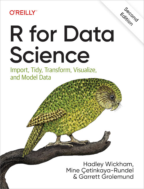
To become efficient in tidying data with R, you are highly encouraged to read through Wickham, Çetinkaya-Rundel, and Grolemund (2023) fifth chapter on data transforms.

Why Choose R for Data Science & DataViz?

1. Free & Open Source

• Zero Cost: 100% free for students, researchers, and institutions worldwide.
• Global Ecosystem: Powered by over 20,000+ open-source CRAN packages.

2. End-to-End Workflow

• Unified Environment: Perform everything from raw data cleaning to statistical modeling and publication-quality graphics without switching tools.
• Reproducibility: Your entire analytical pipeline lives in a single folder.

3. Vibrant Global Community

• Shared Knowledge: Millions of active developers sharing open code, tutorials, and answering questions on StackOverflow, Posit Community, and GitHub.

4. GenAI Precision & Accuracy

• Structured Syntax: Thanks to the consistent grammar of the Tidyverse, modern AI models (ChatGPT, Claude, Copilot) generate remarkably accurate R & {ggplot2} code.

A First Taste of R

The Data Science Workflow

Before diving into details, let us look at the standard analytical workflow in R:

1. Data Import: Loading data into the R environment.
2. Data Wrangling: Cleaning, transforming, and summarizing data into a structure suitable for analysis.
3. Analysis & Visualization: Extracting insights and creating plots to communicate findings.

A First Case Study: Gapminder

We will use the gapminder dataset ({gapminder} package) containing metrics on:

• life expectancy (lifeExp),
• GDP per capita (gdpPercap),
• and population (pop) across countries (country),
• from 1952 to 2007 (year).

Objective

Compute and visualize the average life expectancy and average GDP per capita for each continent across time.

Step 1: Import & Inspect Data

data(gapminder, package = "gapminder")

# Quick look at the first 4 rows
head(gapminder, n = 4)

      country continent year lifeExp      pop gdpPercap
1 Afghanistan      Asia 1952  28.801  8425333  779.4453
2 Afghanistan      Asia 1957  30.332  9240934  820.8530
3 Afghanistan      Asia 1962  31.997 10267083  853.1007
4 Afghanistan      Asia 1967  34.020 11537966  836.1971

Step 2: Data Wrangling {dplyr}

We aggregate statistics by grouping data across continent and year:

library(tidyverse)

gapminder_dplyr <- gapminder |> 
  group_by(continent, year) |> 
  summarise(
    count          = n(),
    mean_lifeexp   = mean(lifeExp),
    mean_gdppercap = mean(gdpPercap),
    .groups        = "drop"
  )

head(gapminder_dplyr, n = 5)

# A tibble: 5 × 5
  continent  year count mean_lifeexp mean_gdppercap
  <fct>     <int> <int>        <dbl>          <dbl>
1 Africa     1952    52         39.1          1253.
2 Africa     1957    52         41.3          1385.
3 Africa     1962    52         43.3          1598.
4 Africa     1967    52         45.3          2050.
5 Africa     1972    52         47.5          2340.

Step 3: Visualization {ggplot2}

ggplot(
  data = gapminder_dplyr,
  mapping = aes(
    x = mean_gdppercap, y = mean_lifeexp,
    color = continent, size = count
  )
) +
  geom_point(alpha = 0.5) +
  labs(
    x = "Average GDP per capita",
    y = "Average life expectancy", 
    color = "Continent",
    size = "No. countries"
  ) +
  theme_minimal(base_size = 14)

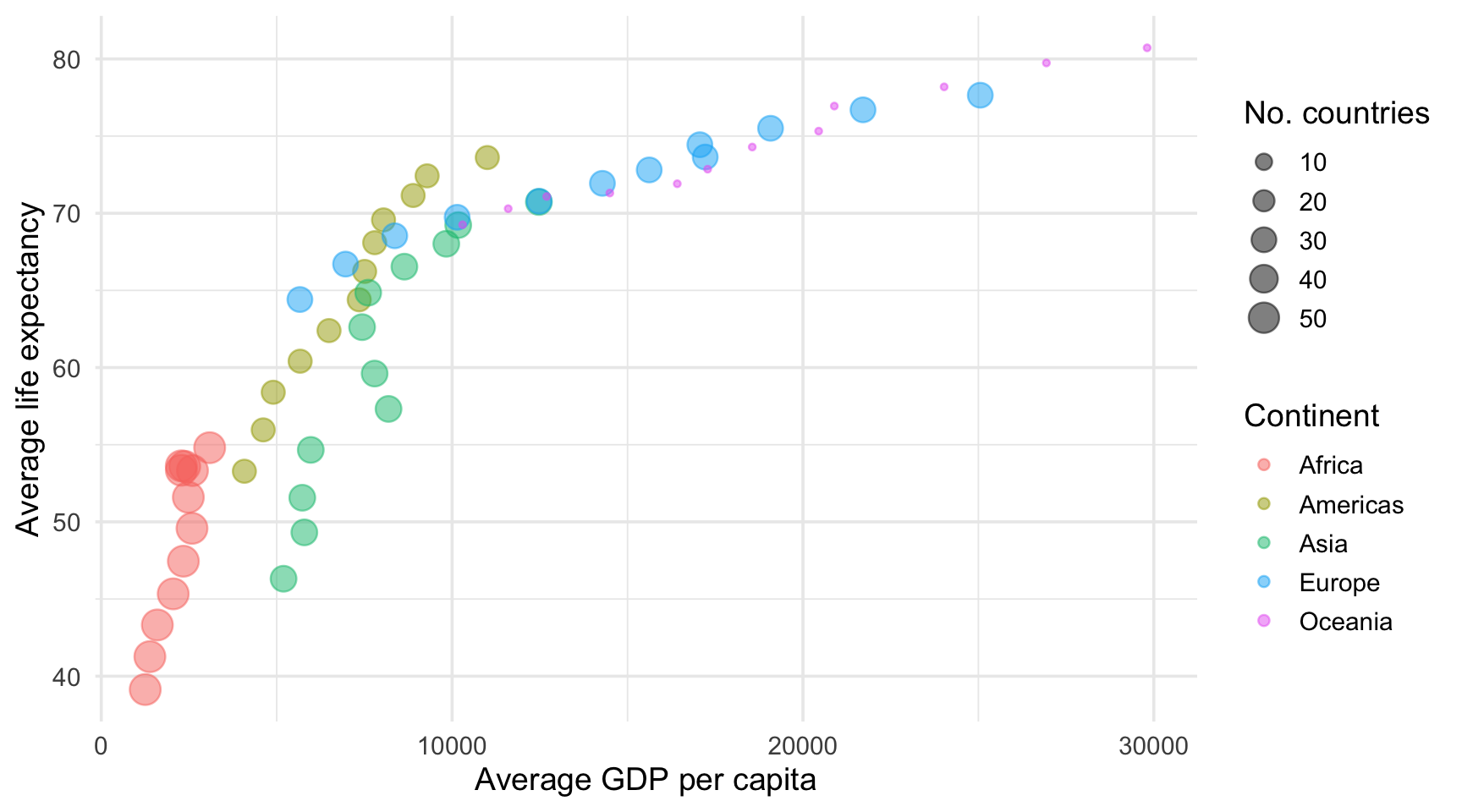
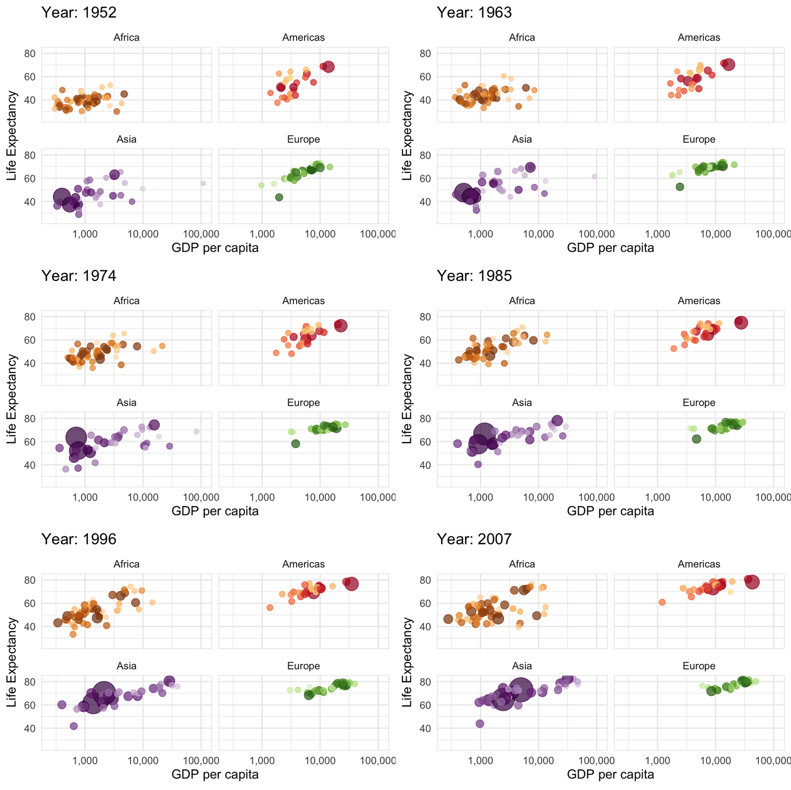
Step 3 (Extended): Animation with {ggplot2} and {gganimate}

library(gganimate)

anim <- ggplot(
  data = gapminder |> filter(continent != "Oceania"),
  aes(gdpPercap, lifeExp, size = pop, color = country)
) +
  geom_point(alpha = 0.7, show.legend = FALSE) +
  scale_colour_manual(values = country_colors) + # (from {gapminder})
  scale_size(range = c(2, 12)) +
  scale_x_log10("GDP per capita", label = scales::comma) +
  facet_wrap(~ continent) +
  theme_minimal(base_size = 14) +
  theme(panel.border = element_rect(color = "grey90", fill = NA)) +
  ylab("Life Expectancy") +
  # Parts which control the animation
  labs(title = "Year: {frame_time}") +
  transition_time(year) +
  ease_aes("linear")

animate(
  anim,
  renderer = gifski_renderer(
    file = "figs/data-wrangling/gapminder_animated.gif"
  ),
  height = 4, width = 6, units = "in", res = 150
)

Source

This animation is taken from Ed Rubin.

R 101: An Express Recap

Glossary

• R: A programming language and software environment for statistical computing and graphics.
• RStudio: An Integrated Development Environment (IDE) designed to work with R efficiently.
• Command / Instruction: User input (text or numbers) that R interprets and executes.
• Script: A text file containing a sequence of commands, executed line by line.
• Working directory: The default folder on your computer where R looks to read files and saves any generated output.

Executing Code from a Script

To evaluate instructions from a script in RStudio:

• Single instruction: Place the cursor anywhere on the line and press Ctrl + Enter (Windows/Linux) or Cmd + Enter (Mac).
• Multiple instructions: Highlight the relevant code lines and press Ctrl + Enter / Cmd + Enter.

RStudio Layout

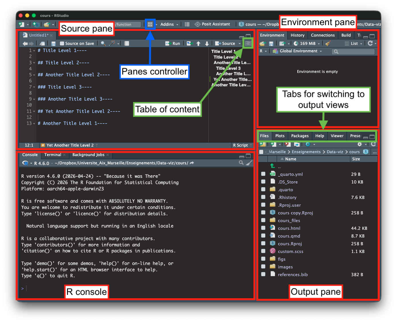
The user interface in RStudio has 4 primary panes:

• Source pane: Where your scripts and documents are written and edited.
• Console pane: Where instructions are evaluated immediately (not saved to a script).
• Environment pane: Displays active R objects, datasets, and functions in the session.
• Output pane: Shows the file explorer, rendered plots, packages, and help docs.

R as a Calculator

• Basic Arithmetic: The R console functions directly as an interactive calculator.
• The Prompt (>): Indicates R is ready for an instruction. Type a command and press Enter.

4 + 1

[1] 5

8 / 2

[1] 4

2^3

[1] 8

• Comments (#): R ignores any text following # on the same line.

# Everything following the '#' is ignored by R
1 + 1 # Code prior to the '#' is executed normally

[1] 2

Task 1: R Project & First Commands

1. Create a dedicated folder for this course on your computer.
2. Open RStudio and create a new project: File \(\rightarrow\) New Project \(\rightarrow\) New Directory \(\rightarrow\) New Project.
   • Name the directory lectures.
   • Click Browse, select your course folder, click Open, then Create Project.

Why use .Rproj files?

RStudio creates an .Rproj file. Double-clicking this file in the future opens RStudio with your working directory automatically set to this project folder.

Task 1: R Project & First Commands

3. Open a new script (File \(\rightarrow\) New File \(\rightarrow\) R Script) and save it as scripts/lecture_intro.R.

4. Type and run the following code in your script:

4 * 8

5. Type and run the following code. What happens if you only execute the first line?

x <- 5
x

Note

Object Assignment

In R, objects are created and assigned using <- (preferred) or =. Everything in R is an object!

6. Create a new object named x_cube and assign it the cube of x.

Help! I need somebody, Help! Not just anybody, Help!

To get some help with R:

1. R built-in functions

?log #? in front of function
help(lm) # help() is equivalent
??plot # get all help on keyword "plot"

2. Read the errors returned. This may be intimidating, but many times, the solution is given in the message returned by the error.

3. Use your favorite search engine (Google, DuckDuckGo, Quant, …): “how to {xxx} in R?”

4. Use your favorite gen AI chatbot (Gemini, Claude, Chatgpt, …): “how to {xxx} in R?” (you can also copy/paste the error to the bot)

5. Use stackoverflow!

R Packages

• R Packages are bundles of add-on functions, documentation, help pages, vignettes, and sample datasets that extend base R.
• Installing Packages:: Executed once per machine.
  • From CRAN: install.packages("kableExtra")
  • From GitHub: remotes::install_github("hadley/YELLING") or pak::pak("hadley/YELLING")
• Loading Packages: Executed once per R session to access its functions:

library(tidyverse)

R Data Types

• Numeric: Continuous numbers or integers (e.g., 42, 3.14, 3L).
• String / Character: Text enclosed in quotes, e.g., "1 string can contain any character!".
• Logical: Boolean values (TRUE, FALSE).
• Missing Values (NA): Represent unobserved or missing entries across any data type.

Checking Data Types in R

Use is.*() helper functions to test the data type of vectors or variables:

• is.numeric(): Checks if a vector is numeric (TRUE for double or integer).
• is.character(): Checks if a vector contains text strings.
• is.logical(): Checks for boolean TRUE/FALSE values.
• is.na(): Identifies missing values. (Crucial: never use x == NA to test for missingness!)

is.numeric(42)       # TRUE

[1] TRUE

is.na(3.14)          # TRUE

[1] FALSE

is.character("hello")# TRUE

[1] TRUE

is.logical(TRUE)     # TRUE

[1] TRUE

Overview of Main Structures

Structure	Dimensions	Homogeneous Types?	Common Use Case
Vector	1D	Yes	Sequences, single variables, series of numbers
List	1D	No	Storing mixed data types, model outputs, nested data (list of list..)
Matrix	2D	Yes	Storing numbers in a 2D table, e.g., for a regression analysis
Data Frame / Tibble	2D	No (mixed across columns, same within)	Rectangular tabular data (rows = observations, columns = variables)

Structures: Vectors

• Creation with c():

c(1, 3, 5, 7, 9)

[1] 1 3 5 7 9

• Coercion to a Single Type:

(v <- c(42, "Statistics", TRUE))

[1] "42"         "Statistics" "TRUE"      

• Generating Sequences:

seq(1, 5, by = 0.5)

[1] 1.0 1.5 2.0 2.5 3.0 3.5 4.0 4.5 5.0

seq(0, 1, length.out = 11)

 [1] 0.0 0.1 0.2 0.3 0.4 0.5 0.6 0.7 0.8 0.9 1.0

1:10

 [1]  1  2  3  4  5  6  7  8  9 10

• Accessing Elements ([]):

x <- 10:20
x[2]

[1] 11

x[c(2, 4)]

[1] 11 13

Structures: Data Frames

• Created with data.frame() by defining column names and assigning vectors of row values:

example_data <- data.frame(
  x = c(1, 3, 5, 7),
  y = c(rep("Hello", 3), "Goodbye"),
  z = c("one", 2, "three", 4),
  alpha = seq(0, 1, length.out = 4),
  beta = letters[1:4]
)
example_data

  x       y     z     alpha beta
1 1   Hello   one 0.0000000    a
2 3   Hello     2 0.3333333    b
3 5   Hello three 0.6666667    c
4 7 Goodbye     4 1.0000000    d

• 2D Structure: Consists of two dimensions (rows and columns).
• Real-World Usage: Typically, datasets are imported from external sources (e.g., CSV, Excel) directly into a data frame rather than created manually.

Using Functions

• Functions are identified by trailing parentheses (). We have already used functions like install.packages(), seq(), and "["().
• The values passed inside parentheses are called arguments. They provide input to the function.
• Functions throw an error if mandatory parameters (required arguments) are missing:

mean()

Error in `mean.default()`:
! argument "x" is missing, with no default

• Pass data to the required argument x to provide values:

mean(x = c(1, 3, 5, 7, 8, 9))

[1] 5.5

Functions & Positional Arguments

Positional Arguments

Because x is the first parameter in mean(), parameter names can be omitted when supplying inputs in exact order:

mean(c(1, 3, 5, 7, 8, 9))

[1] 5.5

Function Outputs & Assignments

• Functions can return multifaceted objects containing far more than single numbers (e.g., outputs from lm(), for linear models).
• Store the output of a function by assigning it to a new object:

my_summary <- summary(c(1, 3, 5, 7, 8, 9))

Assignment Behavior

Assigning output to an object using <- or = suppresses console output. Call the object directly to display its contents:

my_summary

   Min. 1st Qu.  Median    Mean 3rd Qu.    Max. 
   1.00    3.50    6.00    5.50    7.75    9.00 

Checking Object Dimensions

The following built-in functions can be used to inspect the size and shape of R structures:

• length(): Returns the number of elements in a vector/list, or the number of columns in a data frame.
• dim(): Returns a vector with c(rows, columns) for 2D objects (data frames, matrices). Returns NULL for 1D vectors.
• nrow() & ncol(): Return the exact number of rows or columns directly.

Applying those to the iris dataset from {datasets}:

length(iris) # since iris is a data.frame: 5 columns

[1] 5

dim(iris)       # 150 rows, 5 columns

[1] 150   5

nrow(iris)      # 150 rows

[1] 150

ncol(iris)      # 5 columns

[1] 5

Task 2: Data Import & Exploration

1. Find out (using help() or a search engine) how to import a .csv file in R using base R ({utils}). Do not use the “Import Dataset” GUI button in RStudio.
2. Download the law school dataset (Wightman 1998) from https://github.com/fer-agathe/sequential_transport/raw/main/data/law_data.csv.
   • Either download it manually and save it in ./data/, or download it using a function from {utils}.
3. Import the dataset into R using the function from Question 1 and assign it to an object named law.
4. Verify that law is a data frame by evaluating:

class(law)

5. Check the variable names contained in law:

names(law)

6. Inspect the dataset contents by running View(law) or by clicking on law in the Environment pane.

Comparison Operators

Comparison operators evaluate conditions across vectors, matrices, data frames, and lists, returning TRUE or FALSE.

Operator	Description	Example	Result
<	Less than	5 < 10	TRUE
>	Greater than	5 > 10	FALSE
<=	Less than or equal to	10 <= 10	TRUE
>=	Greater than or equal to	5 >= 10	FALSE
==	Exactly equal to	5 == 5	TRUE
!=	Not equal to	5 != 5	FALSE

Logical Operators

Logical operators combine or evaluate boolean statements (TRUE or FALSE).

Operator / Function	Description	Example	Result
&	Element-wise AND	c(TRUE, TRUE) & c(TRUE, FALSE)	TRUE FALSE
|	Element-wise OR	c(TRUE, FALSE) | c(FALSE, FALSE)	TRUE FALSE
!	Logical NOT	!TRUE	FALSE
any()	Returns TRUE if at least one element is TRUE	any(c(FALSE, TRUE))	TRUE
all()	Returns TRUE if every element is TRUE	all(c(TRUE, FALSE))	FALSE

Comparison & Logical Operators in Action

• Comparison Operators on Vectors:

x <- c(12, 18, 25, 30, 45)

# Element-wise comparisons
x > 20

[1] FALSE FALSE  TRUE  TRUE  TRUE

x == 18

[1] FALSE  TRUE FALSE FALSE FALSE

x != 30

[1]  TRUE  TRUE  TRUE FALSE  TRUE

• Subsetting with Conditions:

# Extract elements where condition is TRUE
x[x >= 25]

[1] 25 30 45

• Logical Operators (&, |, !):

# Vectorized AND & OR
(x > 15) & (x < 35)

[1] FALSE  TRUE  TRUE  TRUE FALSE

(x < 15) | (x > 40)

[1]  TRUE FALSE FALSE FALSE  TRUE

# Logical NOT
!(x == 18)

[1]  TRUE FALSE  TRUE  TRUE  TRUE

• Summary Functions (any(), all()):

any(x > 40)

[1] TRUE

all(x > 20)

[1] FALSE

Finding Indices with which()

The which() function takes a logical vector and returns the numeric indices (position numbers) where the condition evaluates to TRUE.

• Logical Condition vs. which():

age <- c(18, 25, 15, 30, 21)

# Returns a logical vector (TRUE/FALSE)
age >= 21

[1] FALSE  TRUE FALSE  TRUE  TRUE

# Returns the index positions where TRUE
which(age >= 21)

[1] 2 4 5

• Useful Variations: which.min() and which.max() return the index of the first minimum or maximum value.

which.min(age)

[1] 3

which.max(age)

[1] 4

Accessing & Editing Data Frames

• Accessing Elements ([rows, cols]):

# Access by column name
example_data[, "y"]

[1] "Hello"   "Hello"   "Hello"   "Goodbye"

# Equivalent options: example_data$y or example_data$`y`

example_data[c(2, 4), c("alpha", "y")]

      alpha       y
2 0.3333333   Hello
4 1.0000000 Goodbye

• Modifying Elements:

example_data[2, "x"] <- -10
example_data

    x       y     z     alpha beta
1   1   Hello   one 0.0000000    a
2 -10   Hello     2 0.3333333    b
3   5   Hello three 0.6666667    c
4   7 Goodbye     4 1.0000000    d

• Adding Columns with $:

example_data$t <- 1:nrow(example_data)
example_data$v <- LETTERS[1:nrow(example_data)]
example_data

    x       y     z     alpha beta t v
1   1   Hello   one 0.0000000    a 1 A
2 -10   Hello     2 0.3333333    b 2 B
3   5   Hello three 0.6666667    c 3 C
4   7 Goodbye     4 1.0000000    d 4 D

Removing Elements From Data Frames

• Removing Columns (NULL or Exclusion):

example_data$t <- NULL
example_data[, c("z", "v")] <- NULL

# Exclude specific column names
example_data <- example_data[, -which(colnames(example_data) %in% c("alpha", "beta"))]
example_data

    x       y
1   1   Hello
2 -10   Hello
3   5   Hello
4   7 Goodbye

• Removing Rows by Index:

example_data <- example_data[-c(1, 3), ]
example_data

    x       y
2 -10   Hello
4   7 Goodbye

Removing Elements From Data Frames

• Data Frame Row Subsetting:

# Find row indices matching condition
matching_rows <- which(example_data$x > 0)

# Use indices to subset
example_data[matching_rows, ]

  x       y
4 7 Goodbye

Handling NA Values

Unlike standard logical indexing (which keeps NA as NA in subsets), which() automatically drops NA positions, returning only valid TRUE indices.

Task 3: Dataset Inspection & Subsetting

1. How many observations are there in the law dataset?
2. How many variables are there? What are the data types of each variable? (in addition to the previously shown functions, you can use str() or glimpse()).
3. Create a new object, law_2, containing only rows 10 to 25 of law.
4. Create a new object, law_3, which contains only the columns sex and UGPA.
5. Add a new column named is_non_white to law to identify non-white individuals by executing:

law$is_non_white <- law$race != "White"

Congratulations, you have created a new variable! Inspect law using head(law) or View(law) to observe the addition.

References

Schwabish, Jonathan A. 2014. “An Economist’s Guide to Visualizing Data.” Journal of Economic Perspectives 28 (1): 209–34. https://doi.org/10.1257/jep.28.1.209.

Wickham, Hadley, Mine Çetinkaya-Rundel, and Garrett Grolemund. 2023. R for Data Science, 2nd Edition. O’Reilly Media, Inc.

Wightman, Linda F. 1998. “LSAC National Longitudinal Bar Passage Study. LSAC Research Report Series.” In. https://api.semanticscholar.org/CorpusID:151073942.