1 Introduction
This document is mainly constructed using different references, including :
- books : Briggs (2013), Grus (2015), VanderPlas (2016), McKinney (2017) ;
- (excellents) notebooks : Navaro (2018).
1.1 Background information
Python is a multiplatform programming language, written in C, under a free license. It is an interpreted language, i.e., it requires an interpreter to execute commands, and has no compilation phase. Its first public version dates from 1991. The main programmer, Guido van Rossum, had started working on this programming language in the late 1980s. The name given to the Python language comes from the interest of its main creator in a British television series broadcast on the BBC called “Monty Python’s Flying Circus”.
The popularity of Python has grown strongly in recent years, as confirmed by the survey results provided since 2011 by Stack Overflow. Stack Overflow offers its users the opportunity to complete a survey in which they are asked many questions to describe their experience as a developer. The results of the 2019 survey show a new breakthrough in the use of Python by developers. As shown in Figure 1.1 41.1% of respondents indicate that they develop in Python, i.e., 2.3 percentage points higher than a year earlier.
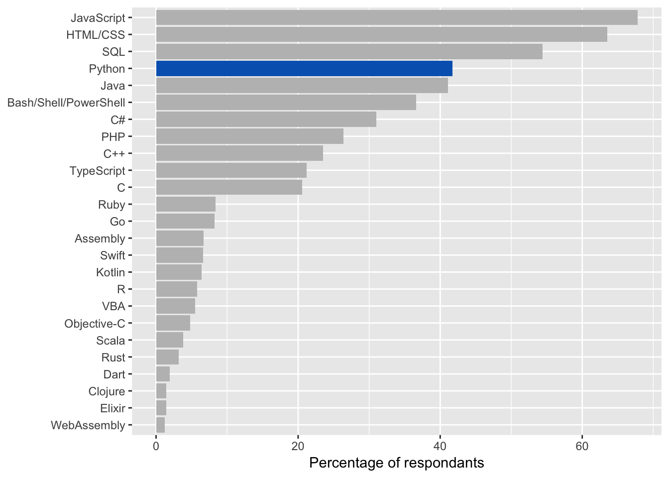
Figure 1.1: Programming, Scripting, and Markup Languages.
1.2 Versions
These course notes are intended to provide an introduction to Python, version 3.x. In this sense, the examples provided will correspond to this version, not to the previous ones.
Compared to version 2.7, version 3.0 has made significant changes. It should be noted that Python 2.7 will take “its retirement” on January 1, 2020. After this date, support will no longer be provided.
1.3 Working space
There are many environments in which to program in Python. We will briefly present some of them.
It is assumed here that you have installed[Anaconda] (https://www.anaconda.com/) on your computer. Anaconda is a free and open source distribution of the Python and R programming languages for data science and machine learning applications. In addition, when the terminal is mentioned in the notes, it is assumed that the operating system of your machine is either Linux or Mac OS.
1.3.1 Python in a terminal
It is possible to call Python from a terminal, by executing the following command (under Windows: in the start menu, launch the “Python 3.6” software):
pythonWhat can be seen on screen is reproduced in Figure 1.2 :
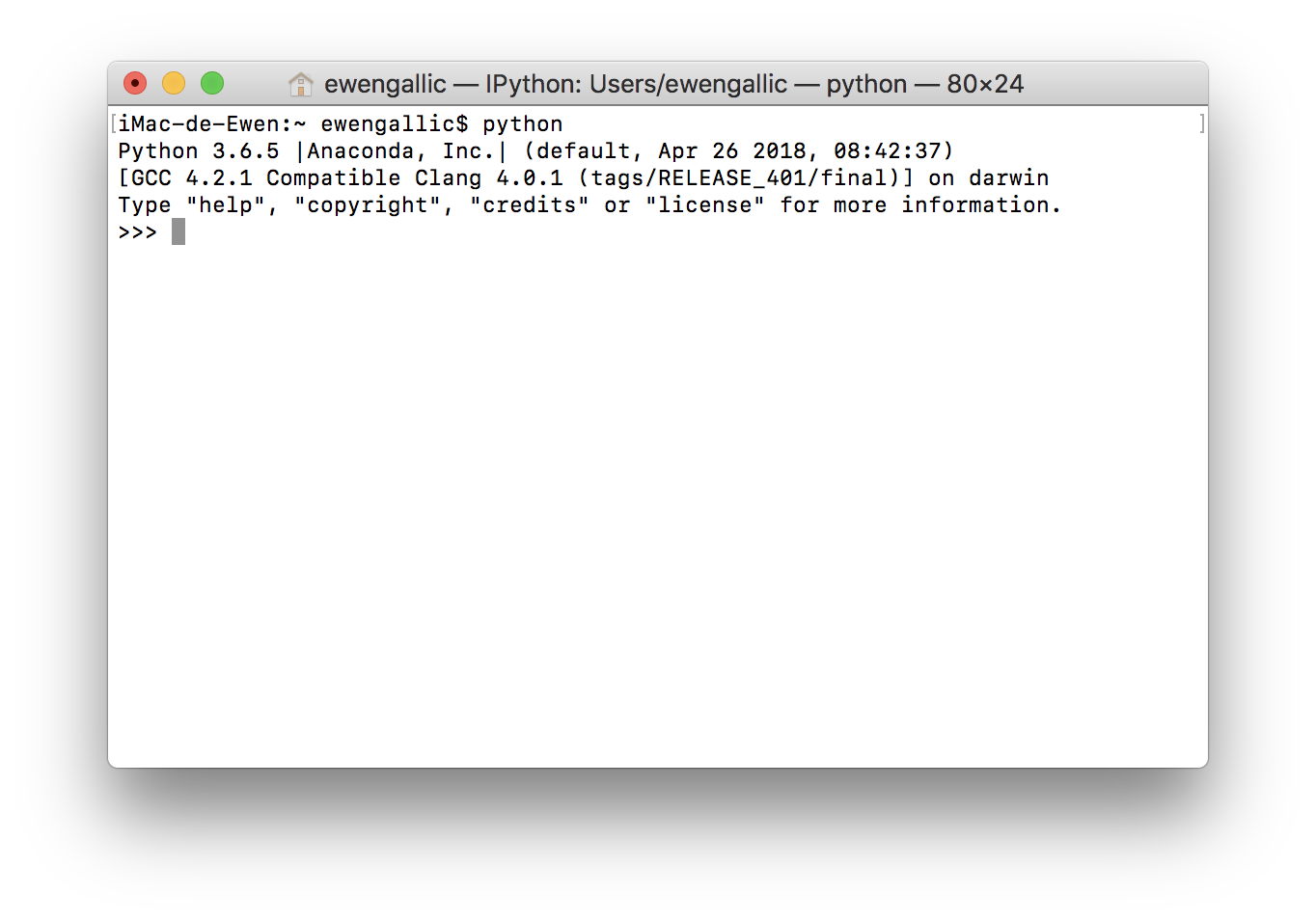
Figure 1.2: Python in a terminal.
We note the presence of the characters >>>> (prompt), which invite the user to enter a command. Expressions are evaluated once they are submitted (using the `ENTEREE’ key) and the result is given, when there is no error in the code.
The presence of the characters >>> (prompt), which invite the user to enter a command can be noticed. Expressions are evaluated once they are submitted (using the `ENTER’ key) and the result is given, when there is no error in the code.
For example, when evaluating 2+1:
>>> 2+1
3
>>>
The prompt at the end can be noted: this tells the user that Python is ready to receive new instructions.
1.3.2 IPython
There is a slightly more friendly environment than Python in the terminal: IPython. It is also an interactive terminal, but with many more features, including syntax highlighting or auto-completion (using the tab key).
IPython can be opened using a terminal, using the following instruction:
ipythonIPython can also be launched from Anaconda’s home window, by clicking on the Launch button of the qtconsole application, visible in the Figure 1.3.
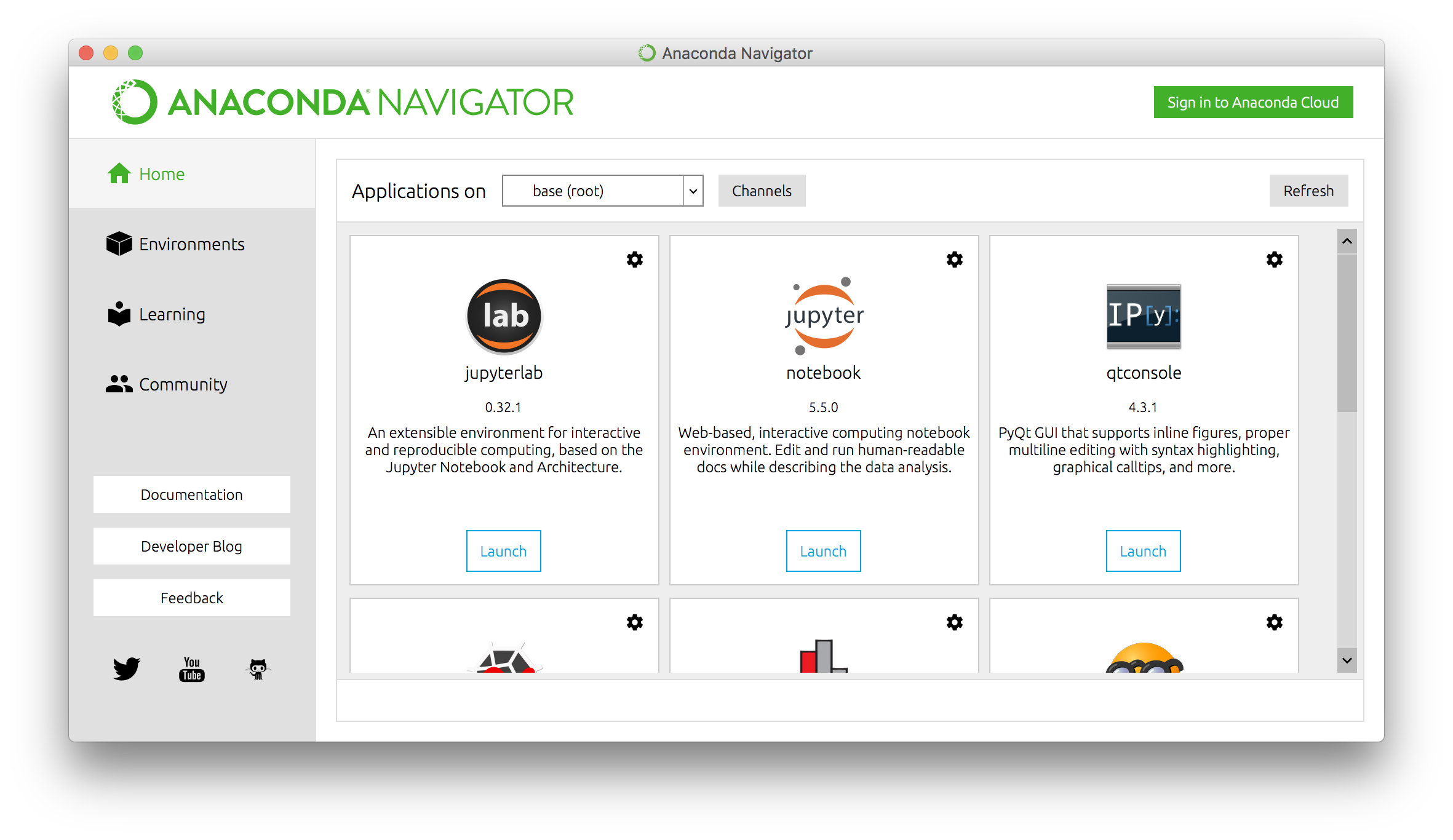
Figure 1.3: Anaconda’s home window.
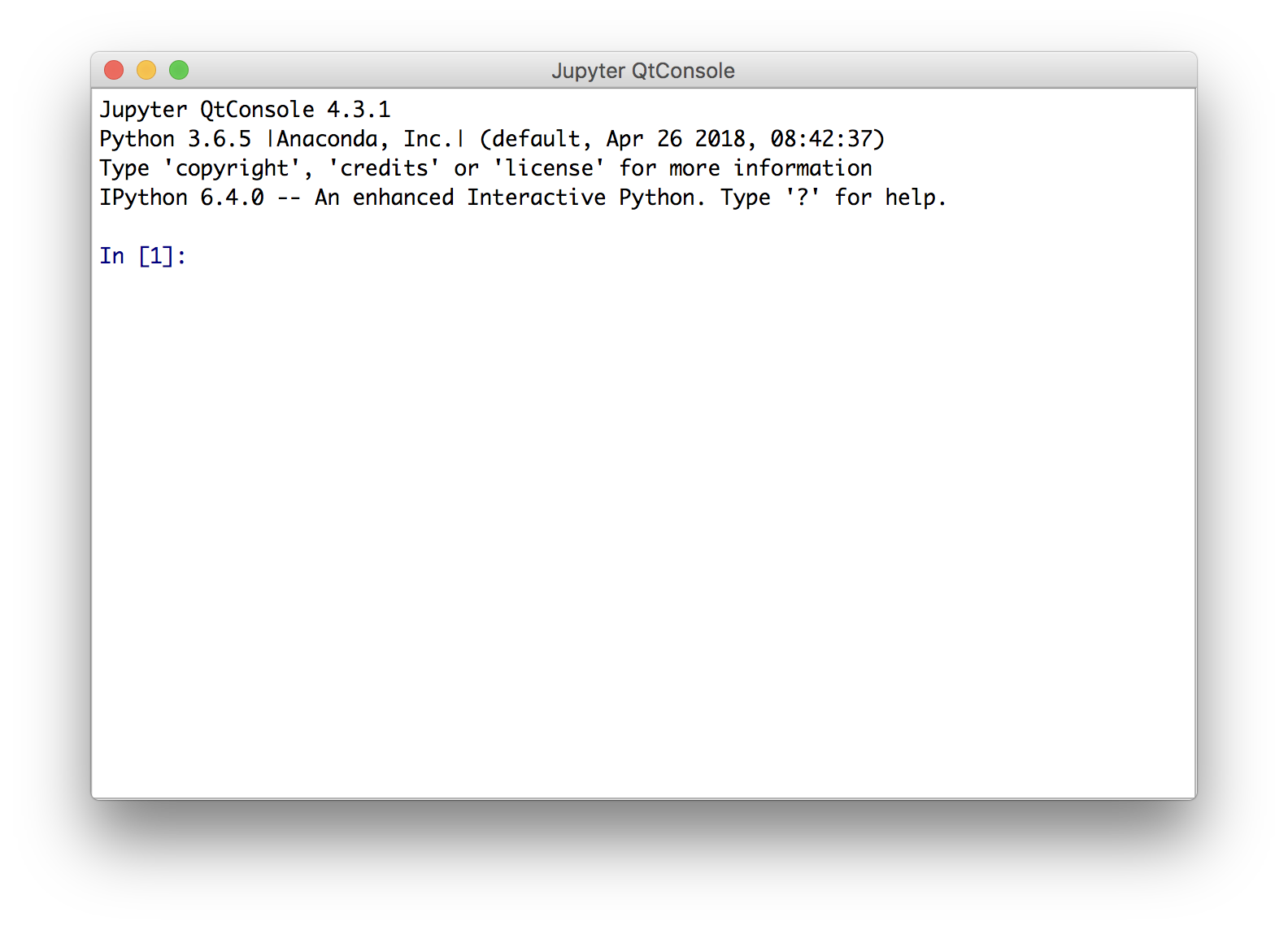
Figure 1.4: IPython console.
Let’s submit a simple instruction:
The results shows:
In [1]: print("Hello World")
Hello World

In [2]:
Several things should be noted. First, we note that at the end of the execution of the instruction, IPython indicates that it is ready to receive new instructions, by the presence of the prompt In[2]:. The number in brackets refers to the instruction number. We note that it went from 1 to 2 after the execution. We also note that the result of the call to the print() function, with the string of characters (delimited by quotation marks), displays on the screen what was contained between the parentheses.
1.3.3 Spyder
While when using Python in a terminal, it is recommended to have a text editor open next to it (to be able to save instructions), such as, for example, Sublime Text for Linux or Mac OS users, or notepad+++ for Windows.
Another alternative is to use a single integrated development environment (IDE) that includes both an editor and a console. This is what Spyder offers, with many additional features, such as project management, file explorer, command log, debugger, etc.
To launch Spyder, one can open a terminal and simply evaluate Spyder (it is also possible to launch the software using the Start Menu for Windows users). Spyder can also be launched via Anaconda.
The development environment, as shown in Figure 1.5, is divided into several windows:
- on the left: the script editor;
- at the top right: a window to display Python help, the system tree or the variables created;
- bottom right: one or more consoles.
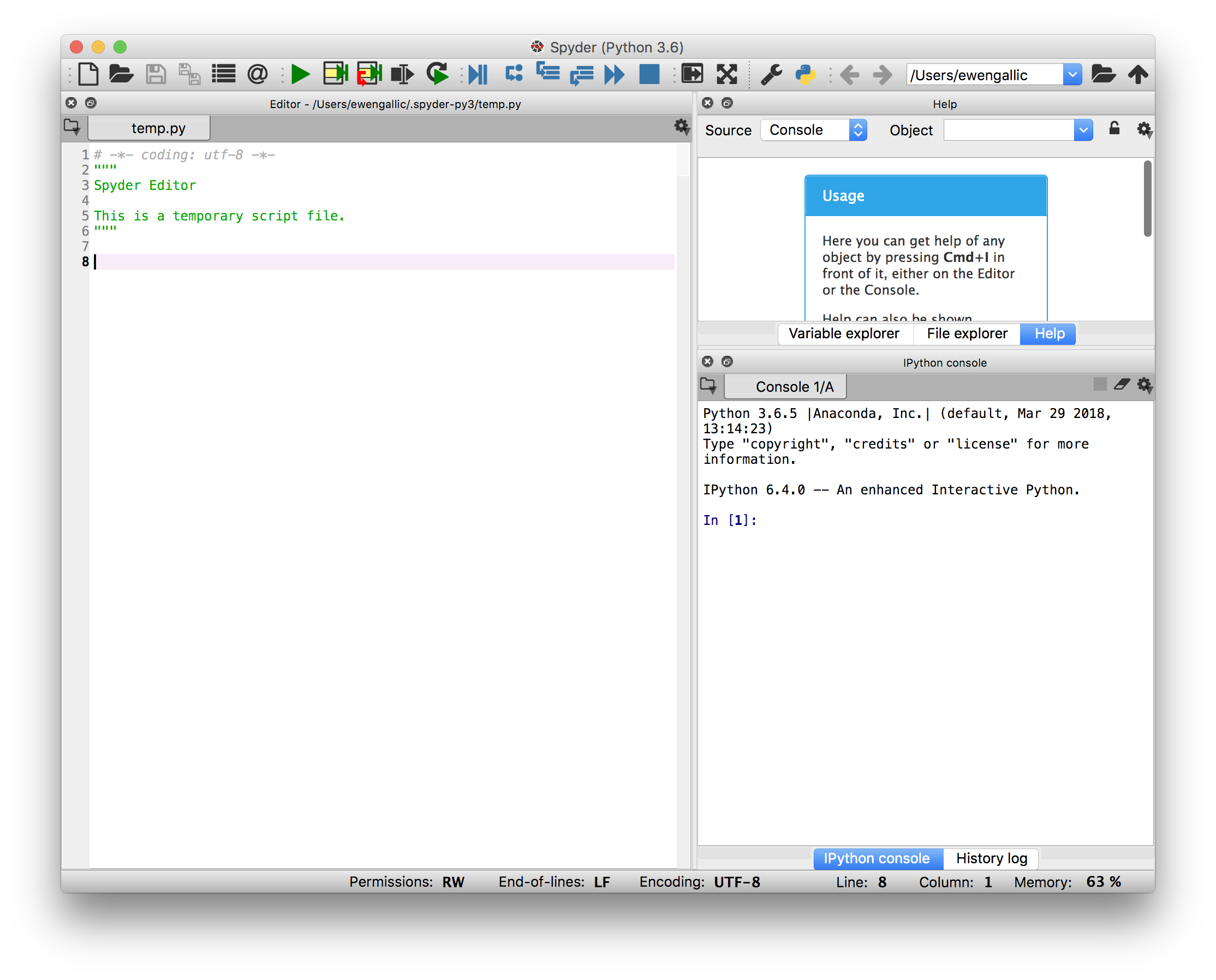
Figure 1.5: Spyder.
1.3.4 Jupyter Notebook
A graphical user interface in a web browser for IPython has gained has gained a strong popularity in the recent years: Jupyter Notebook. It is an open-source application for creating and sharing documents that contain code, equations, graphical representations and text. It is possible to include and execute different language codes in Jupyter notebooks.
Jupyter Notebook can be launched through Anaconda. After clicking on the Launch button of Jupyter Notebook in Anaconda, the default web browser launches and offers a tree structure, as depicted in Figure 1.6. Without realizing it, a local web server was launched as well as a Python process (a kernel).
If the browser does not launch automatically, the page that should have been displayed can be accessed at the following address: http://localhost:8890/tree?.
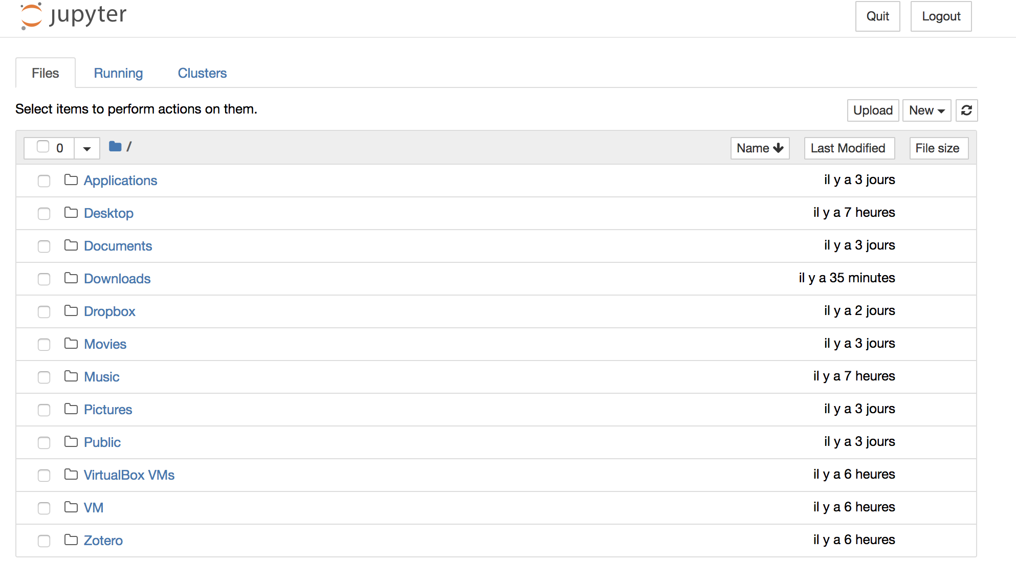
Figure 1.6: Jupyter Notebook.
To address the main functions of Jupyter, create a jupyter folder in a directory of our choice. Once this folder has been created, navigate through the Jupyter tree structure in the web browser.
Once in the folder, create a new Python 3 Notebook (by clicking on the New button at the top left of the window, then on Python 3).
A notebook named Untitled has just been created, the page displays an empty document, as shown in Figure 1.7.
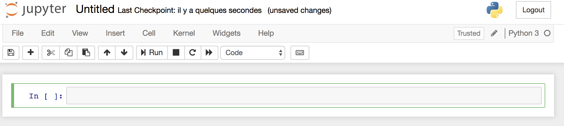
Figure 1.7: An Empty Notebook.
If we look in our file explorer, in the newly created jupyter folder, a new file has appeared: Untitled.ipynb.
1.3.4.1 Evaluation of an instruction
Let us go back to the web browser, to the page displaying your notebook.
Below the menu bar, we notice the presence of a framed area, a cell, that starts with IN []:, like what we saw in the console on IPython. On the right, the grey area invites us to submit instructions in Python.
Let us write the following instruction:
To submit the instruction for evaluation, there are several ways (make sure you have clicked inside the cell):
- in the menu bar:
Cell > Run Cells; - in the shortcut bar: button
Run; - with the keyboard: hold down the
CTRLkey and pressEnter.
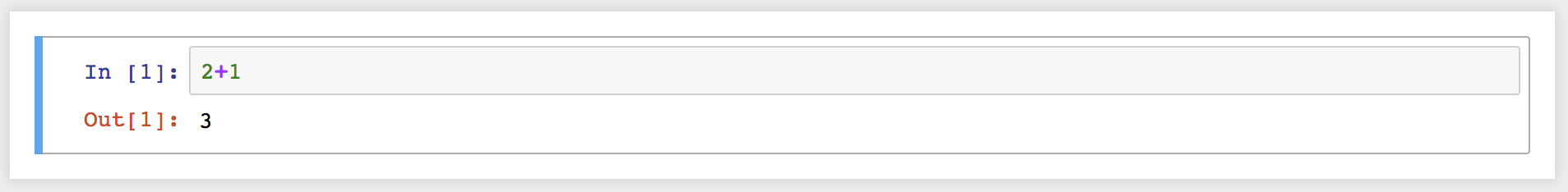
Figure 1.8: Evaluated Cell.
1.3.4.2 Text cells
Among the advantages of notebooks over traditional scripts is the possibility to add text boxes to accompany the codes and the corresponding output after evaluation.
Let’s add a cell below the first one. To do this, one can proceed either:
- using the menu bar:
Insert > Insert Cell Below(to insert a cell below; if you want an insertion above, just chooseInsert Cell Above); - by clicking in the frame of the cell from which you want to add (anywhere except in the grayed out code area, so that you can switch to
command' mode), then pressing theBkey on the keyboard (A` for insertion above).
The new cell calls for a Python instruction to be entered. To indicate that the content should be interpreted as text, it is necessary to specify it. Again, there are several ways to do this:
- using the menu bar:
Cell > Cell Type > Markdown; - using the shortcut bar: in the drop-down menu where
Codeis written, by selectingMarkdown; - in command mode (after clicking inside the cell frame, but not in the code area), by pressing the
Mkey on the keyboard.
The cell is then ready to receive text, written in markdown. For more information on writing in Markdown, you can refer to this [cheat sheet] (https://github.com/adam-p/markdown-here/wiki/Markdown-Cheatsheet).
Let’s enter a few lines of text to see very briefly how the cells written in Markdown work.
# A Level 1 Title

I will write *text in italics* and also **in bold**.

## A Level 2 Title

I can write lists:

- with an item
- a second one
- and a third nesting a new list:
    - with a subitem
    - and a second one
- a fourth one including a numbered nested list:
    1. with a subitem
    1. and another.

## Another Level 2 Title


I can even put equations in $LaTeX$.
Like $X \sim \mathcal{N}(0.1)$.

To learn more about $\LaTeX$, we can refer to this :
  [Wikipedia page](https://en.wikibooks.org/wiki/LaTeX/Mathematics).
Which gives, in Jupyter:
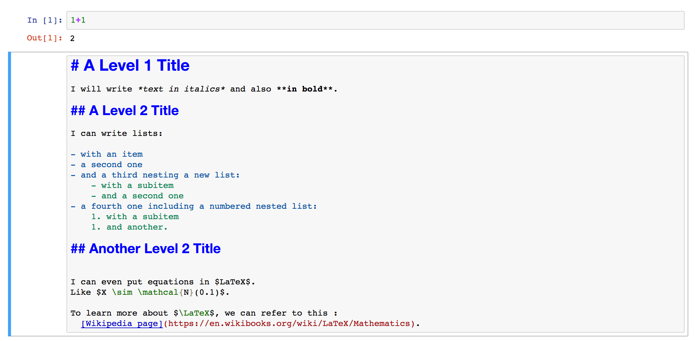
Figure 1.9: Text cell not evaluated.
Then, the cell still has to be evaluated, as if it were a cell containing a Python instruction, to switch to a Markdown display (CTRL and ENTER).
To edit the text once we have switched to markdown, a simple double-click in the cell text box does the trick.
To change the cell type so that it becomes code:
- using the menu bar:
Cell > Cell Type > Code; - using the shortcut bar: in the drop-down menu where
Codeis written, by selectingCode; - in command mode, press the key on the
Ykeyboard.
1.3.4.3 Deleting a cell
To delete a cell:
- using the menu bar:
Edit > Delete Cells - using the shortcut bar: scissor icon
- in command mode, press the
Dkeyboard key twice.
1.4 Variables
1.4.1 Assignment and deletion
When we evaluated the 2+1 instructions earlier, the result was displayed in the console, but it was not saved. In many cases, it is useful to keep the content of the result in an object, so that it can be reused later. To do this, variables are used. To create a variable, we use the equality sign (=), followed by what we want to save (text, a number, several numbers, etc.) and preceded by the name we will use to designate this variable.
For example, if we want to store the result of the calculation 2+1 in a variable that we will name x, we write:
To display the value of our variable x, we can use the function print():
## 3To change the value of the variable, a new assignment can be made:
## 4It is also possible to give more than one name to the same content (a copy of x is made):
## 4If the copy is modified, the original will not be affected:
## 0## 4A variable can be deleted with the instruction del:
The display of the content of `y’ returns an error:
## Error in py_call_impl(callable, dots$args, dots$keywords): NameError: name 'y' is not defined
##
## Detailed traceback:
##   File "<string>", line 1, in <module>
But we note that the variable x has not been deleted:
## 41.4.2 Naming Conventions
The name of a variable can be composed of alphanumeric characters as well as the underscore (_) (there is no limit on the length of the name). It is forbidden to start the name of the variable with a number. It is also prohibited to include a space in the name of a variable.
To increase the readability of the variable names, several methods exist. We will adopt the following:
- all letters in lowercase;
- the separation of terms by an underscore (
_).
For example, for a variable containing the value of a user’s identifier: id_user.
It should be noted that the variable names are case sensitive:
## toto## Error in py_call_impl(callable, dots$args, dots$keywords): NameError: name 'X' is not defined
##
## Detailed traceback:
## File "<string>", line 1, in <module>1.6 Modules and packages
Some basic functions in Python are loaded by default. Others require a module to be loaded. These modules are files that contain definitions as well as instructions.
Package are defined as a combination of modules that offer a set of functions.
Among the packages that will be used in these notes are:
- NumPy, a fundamental package for scientific calculations
- pandas, a package allowing easy data manipulation and analysis
- Matplotlib, a package allowing us to create graphics.
To load a module (or a package), we use the command import. For example, to load the package pandas:
This allows us to use functions contained in the module or package. For example, here we can use the function Series(), contained in the package pandas, to create an array of data indexed to a dimension :
## 0    1
## 1    5
## 2    4
## dtype: int64
It is possible to give an alias to the module or package that is imported, by specifying it using the following syntax:
This is common practice to shorten the names of modules that will be used a lot. For example, for pandas, the name is usually shortened to pd:
## 0    1
## 1    5
## 2    4
## dtype: int64
A single function can also be imported from a module, and an alias can be assigned to it (optionally). For example, with the pyplot() function of the package matplotlib, we usually do the following:
import matplotlib
import matplotlib.pyplot  as plt
import numpy  as np
x = np.arange(0, 5, 0.1);
y = np.sin(x)
plt.plot(x, y)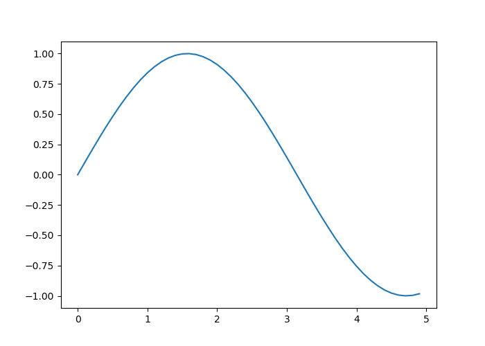
1.7 The Help System
To conclude this introduction, it seems important to mention the presence of help and documentation in Python.
For information on functions, it is possible to refer to the[online documentation] (https://docs.python.org/3/). It is also possible to get help inside the environment we are using, using the question mark (?).
For example, when using IPython (which, let’s remember, is the case when working with Jupyter Notebook), the help can be accessed using different syntaxes:
?: fournitprovides an introduction and an overview of the features offered in Python (you leave it with theESCkey for example)object?: provides details aboutobject(for examplex?orplt.plot?)object??: more details aboutobject%quickref: short reference on Python syntaxeshelp(): access to the Python help system.
Note: the tabulation key on the keyboard allows not only autocompletion, but also an exploration of the content of an object or module.
In addition, when it comes to finding help on a more complex problem, the right thing to do is not hesitate to search on a search engine, in mailing lists and of course on the many questions on Stack Overflow.
References
Briggs, Jason R. 2013. Python for Kids: A Playful Introduction to Programming. no starch press.
Grus, Joel. 2015. Data Science from Scratch: First Principles with Python. " O’Reilly Media, Inc.".
McKinney, Wes. 2017. Python for Data Analysis: Data Wrangling with Pandas, Numpy, and Ipython (2nd Edition). " O’Reilly Media, Inc.".
VanderPlas, Jake. 2016. Python Data Science Handbook: Essential Tools for Working with Data. " O’Reilly Media, Inc.".
1.5 Comments
There are several ways to add comments in python.
One way is to use the number sign (
#) to make a comment on a single line. Everything that follows the number sign to the end of the line will not be evaluated by Python. On the other hand, what comes before the number sign will be.The introduction of a block of comments (comments on several lines) is done by surrounding what is to be commented with a delimiter: three single or double quotation marks: