Introduction to programming for data analysis

Session 2 — Data Wrangling

Ulrich Aiounou

dimitri.aiounou@univ-amu.fr

AMSE, Aix Marseille University

Ewen Gallic

ewen.gallic@univ-amu.fr

AMSE, Aix Marseille University

Disclaimer

The slides were adapted from those of Pierre Michel and Morgan Raux, both researchers at AMSE, who kindly shared their work.
This slide deck was made with Quarto and reveal.js, it is translated by Claude Sonnet 5 from a LaTex presentation previously made with beamer.

The 4 steps in any data analysis

Finding data
Cleaning data to combine several data sources
Producing knowledge out from data (summary statistics, regression analysis summarised via tables and graphs)
Interpreting the results (writing)

Finding data

How can we find data?

Finding the most appropriate data is the most important part of any empirical project!
Although, no one can teach you how to do that.
We can only give you a few tips.
Finding data is very time consuming.
However, spending more time to be sure to find the best possible available data will make each following step easier.

A few advices from Alex the Analyst

🌐 Video on finding data

Primary vs Secondary data

The data we will find on these websites are secondary data.
Secondary data is data that has already been collected, processed, and possibly analyzed by someone else for a different purpose than the current research project.
Primary data is original data collected directly by the researcher or organization for a specific research purpose or project.
You can collect your own primary data through survey collection, web-scraping, digitizing archives.

Description and Aim of the Session

In this session, we want to study the relationship between the geographic distribution of universities and the likelihood to attend college education.
The hypothesis we want to explore is the following:
- Is the presence of a university in the county of residence of a given individual positively associated with the probability that this individual attends university?

Outline of the session

In this session, we are going to:

Find appropriate data to test this hypothesis empirically.
Clean and format the data.
Draw a few summary statistics to illustrate our topic of interest.
Run a few simple regressions to test this hypothesis.
Interpret the results.

Finding data

The first step before coding is always to find the most appropriate data to test our hypothesis empirically.

Question 1: What type of data do we want to test our hypothesis?

Question 2: What could be an appropriate unit of observation in our data to test this hypothesis?

Data strategy

Morgan Raux has collected for you US labor force data for year 2018.
This data covers a representative sample of US workers and includes information on their college education status and the county of residence of their parents.
We now want to find data on the geographic distribution of US universities.
The ideal dataset we want is the list of US colleges with information on their location county.
After finding such data, we can combine the two datasets and test our hypothesis.

Set Your RStudio Project

Root
  data
    raw
    tmp
    out
  functions
  scripts
  notebooks
  figs
  tables
  references
  project.Rproj

Open RStudio
Create a new project
- File → New Project...
- Choose New Directory
- Create a project named session-2
Create the project structure

In the R console, run:

dir.create("data")
dir.create("data/raw")
dir.create("data/tmp")
dir.create("data/out")
dir.create("functions")
dir.create("scripts")
dir.create("notebooks")
dir.create("figs")
dir.create("tables")
dir.create("references")

Exercise

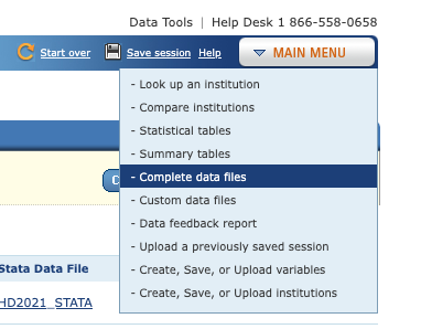
Find the university dataset on the geographic distribution of US universities.
Hint: the US statistical agency collecting data on US higher education is called IPEDS
- use the IPEDS Data Explorer; look for complete data files.
- since we have data from 2018, let us use a survey from the same year.
Once you have downloaded the data, put it in the data/ folder of your project for session 2.

Solution: Link to the Desired Dataset

From the IPEDS website’s homepage, in the menu “Use the data”, click on “Complete Data Files” to access the data explorer tool.
On the main menu of this tool, we need to select “Complete data files”.
After filtering for year 2018, the dataset we are looking for appears, it is called HD2018.
- the dataset in a ZIP file,
- a companion dictionary of variables

Coding Preamble

What are functions? Libraries? and Loops?

Before getting further, we need to see 3 coding concepts that are key for R:

What is a function?
What is a library?
What is a loop?

What is a Function in `R`?

A function in R is a block of organized, reusable code that performs a specific task.
Functions help to make code more modular, readable, and easier to debug and maintain.

Key Components of a Function

A function in R is made of the following components:

Function Name: the name you use to call the function.
Arguments: inputs to the function, specified within parentheses.
Body: a set of statements that define what the function does, enclosed in curly braces {}.
Return Value: the result/output of the function:
- You’ll sometimes see people use the return() function to explicitly state what should be returned.
- By default, the last evaluated expression of the body of the function is returned.
- Hence, return() is mostly used for functions that contain conditional expressions (if...else).

Syntax

function_name <- function(argument_1, argument_2) {
    result <- argument_1 + argument_1 # Example of operation

    result # The last instruction in the body is what is returned
}

Example

#' Addition of two numbers
#' 
#' @param x First number.
#' @param y Second number.
#' @returns The sum of x and y.
add_numbers <- function(x, y) {
    sum <- x + y

    sum
}

# Call the function with arguments:
add_numbers(x = 2, y = 3)

Exercise

Write a function called pct_change() that takes two arguments, old_value and new_value, and returns the percentage change between them.

Recall: percentage change \(= \dfrac{\text{new} - \text{old}}{\text{old}} \times 100\)
Test it with pct_change(old_value = 80, new_value = 100) (it should return 25).

What is a Library in `R`?

A library in R is a collection of functions and associated help pages, (and, optionally, data), and compiled code in a well-defined format.
Libraries (or packages) extend the functionality of R by adding new features.
The most basic functions are in the base package, loaded by default when you launch R.

Key Features of Libraries

Reusable Code
- Libraries contain reusable functions and datasets.
Community Contributions
- Thousands of libraries are available, many contributed by the R community.
Specialized Functions
- Libraries provide specialized tools for specific tasks, such as data manipulation, visualization, machine learning, and more.

Using Libraries in R

Installing a Library:
- Use the install.packages("libraryname") function to install a library.
Loading a Library:
- Use the library(libraryname) function to load an installed library.

Do not mix the two! There is no need to install the library each time you want to use it. Just load it. Here is an analogy:

Installing → downloading the app from the App Store / Google Play.
Loading → tapping the app to open it and use it.
You do not reinstall WhatsApp every time you want to send a message, you just open it.

What is a Loop in R?

A loop in R is a control flow statement that allows code to be executed repeatedly based on a condition.
Loops help to automate repetitive tasks and perform iterations over collections of data.
Each repetition of the instructions of the code is called an iteration.

Types of Loops in R

There are two types of loops:

for loop: iterates over a sequence of elements.
- The computer knows in advance how many iterations this will take.
while loop: repeats a block of code until a condition is met (is TRUE).
- The computer does not know in advance how many iterations this will take.

for Loop Syntax and Example

Syntax:

for (variable in iterable_object) {
    # Instruction(s) to execute
}

Example:

# Print the squares of the integers from 1 to 5
for (i in 1:5) {
    j <- i^2
    print(j)
}

while Loop Syntax and Example

Syntax:

while (condition) {
    # instructions to execute
}

Example:

# Print the squares of the integers until the current integer 
# is lower or equal to 5
i <- 1 # initialize the counter to 1
while (i <= 5) {
    j <- i^2
    print(j)
    i <- i + 1 # Increment the counter
}

Exercise

Write a for loop that prints for each integer from 1 to 10, whether it is even or odd.

Recall: use the modulo operator %% to test divisibility (e.g., i %% 2 == 0 is TRUE when i is even).

Importing data

Manage the Working Directory

To print the path to the current working directory (set by default):

getwd()

The working directory can be assigned by the user using the following command:

setwd("C:/Users/myName") # Windows example

Bad Practice!

Changing manually the working directory is bad practice: when you share your codes, it quickly becomes a nightmare to others who have to modify your scripts to change the working directory on their end.

Use RStudio’s projects instead. The working directory becomes the same as that which contains the .Rproj file.

Importing data

Common data importing functions
- read_csv(), read_delim() from the readr package
- read_excel() from the readxl package
- read_sav(), read_sas(), read_dta() from the haven package
Learn more about importing multiple files at once 🌐 here.

Import text files

To load text files (e.g., the age_gender.txt files stored in your computer, use the function read.table().

read.table(file, sep, header)

file: the name of the file (character)
sep: separator used in file (” ” by default)
header: TRUE if file contains column names, FALSE by default

tab <- read.table(file = "data/age_gender.txt", header = TRUE)
head(tab, 3)

age	gender
28	F
36	H
45	F

Import text files: variants of read.table()

file.choose(): choose a file through the GUI.
read.csv(): read CSV files.
read.delim(): read delimited text files.
read.fwf(): read fixed-width-formatted files.

R can read files in specific software formats (Excel, SAS, SPSS, Stata) using the functions from the foreign package.

# Try this
install.packages("foreign")
library(foreign)
?read.dta

Export text files

To export a data.frame into text files in your working directory: write.table().

write.table(x, file, append, col.names, row.names)

x: data.frame.
file: name of the file in which to write.
append: if TRUE, add to an (eventually existing) file, if FALSE, overwrite the existing file (default).
col.names and row.names: if TRUE, write the columns/rows names.

write.table(tab, "age_gender.txt", row.names = TRUE,
col.names = TRUE)

💡 write() is similar to write.table(), with fewer options.

Save/Load R objects

R objects can be saved in both ascii and binary formats:

dump(): save R objects in ascii format.
source(): load R objects saved with dump().
save(): save R objects in binary format.
load(): load R objects saved with save().

# Try this
dump(ls(), file = "objects.txt")
source("objects.txt")

save(iris, mtcars, file = "iris_and_mtcars.rda")
load("iris_and_mtcars.rda")

Exercise: Import

Import the HD2018.csv file you downloaded from IPEDS into an object called universities.
Also import the labor force survey data, available on AMeTICE (Moodle) as US_labor_force_survey.dta, into an object called survey. Use the following instruction:

  survey <- haven::read_dta("data/US_labor_force_survey.dta")

Put both files in the data/ folder of your project for session 2 before importing them.

Solution: Import

library(tidyverse)
# University dataset (CSV)
universities <- read_csv("data/HD2018.csv")

# Labor force survey (Stata format)
survey <- haven::read_dta("data/US_labor_force_survey.dta")

read.csv() (base R) or readr::read_csv() both work for the .csv file; the latter is faster and returns a tibble.
haven::read_dta() is needed for the .dta file, since Stata’s binary format is not plain text.

What is a Clean Dataset?

Data are ready

Six Data quality indicators

Analyzable
Interpretable
Complete
Valid
Accurate
Consistent

Analyzable

Data should make a rectangle of rows and columns.
The first row, and only the first row, is your variable names (otherwise: skip).
The remaining data should be made up of values in cells.
At least one column uniquely defines the rows in the data (e.g., unique identifier).

Analyzable

Column values are analyzable.
Information is explicit.

Analyzable

Only one piece of information is collected per variable.

Otherwise: separate_rows().

Exercise

What data quality issues do you detect for the analyzable indicator?

Solution

Data do not make a rectangle.
Color coding used to convey information.
More than one piece of information in a variable.
Blank values implied to be 0 for Q4 variables.

Interpretable

Variable names should be machine-readable:
- Unique.
- No spaces or special characters except underscore (_),
  - This includes no dot (.) or hyphen (-),
- Not begin with a number (should begin with a letter),
- Character limit of 32 is better.
Variable names should be human-readable:
- Meaningful (gender instead of X1),
- Consistently formatted (capitalization and delimiters),
- Consistent order of information.

Exercise

What data quality issues do you detect for the interpretable indicator?

Solution

Spaces and special characters used in variable names.
Some variable names are unclear.
Inconsistent use of capitalization.

Complete

Observations
- The number of rows in your dataset should sum to your sample size \(N\) (excluding header):
  - No missing observations,
  - No duplicate observations (i.e., no unique identifier repeated).
Variables
- The number of columns in your dataset should total to what you planned to have:
  - No missing variables,
  - No unexpected missing data,
  - If you collected the data, it should exist in the dataset.

Exercise

What data quality issues do you detect for the complete indicator?

Solution

The data contain a duplicate ID (104).

Valid

Variables conform to the planned constraints:
- Planned variable types (e.g., numeric, character, date),
- Allowable variable values and ranges (e.g., \([1,5]\)),
- For surveys: item-level missingness aligns with variable universe rules and skip patterns.

Exercise

What data quality issues do you detect for the valid indicator?

Solution

AGE/YR does not adhere to our planned variable type.
Values in Score fall out of our expected range.

Accurate

Information should be accurate based on any implicit knowledge you have.
- For instance, maybe you know a student is in 2nd grade because you’ve interacted with that student, but their grade level is shown as 5th in the data.
Accurate within and across sources
- A date of birth collected from school records should match the date of birth provided by the student.
- If a student is in 2nd grade, they should be associated with a second grade teacher.

Exercise

What data quality issues do you detect for the accurate indicator?

Solution

ID 105 has conflicting information for TEACHING LEVEL and SCHOOL.

Consistent

Variable values must be consistently measured, formatted, or categorized within a column.
Variables must be consistently measured across collections of the same form.

Exercise

What data quality issues do you detect for the consistent indicator?

Solution

Values for GENDER are not consistently categorized.

Recap: Data validation

Complete
- Check for missing/duplicate cases
- Check Ns by groups for completeness
- Check for missing/too many columns
Valid and consistent
- Check for unallowed categories/values out of range
- Check ranges by groups
- Check for invalid, non-unique, or missing study IDs

Consistent
- Check for incorrect variable types/formats
- Check missing value patterns
Accurate
- Agreement across variables
Interpretable
- Variables correctly named

Standard Data Cleaning Checklist

Import the raw data
Review the raw data
Find missing data
Adjust the sample
Drop irrelevant columns
Split columns
Rename variables
Normalize variables

Standardize variables
Update variable types
Recode variables
Construct new variables
Validate data
Join datasets
Reshape data
Save clean data

Data Preparation with R

Working with the HD2018 dataset

We will be working on the HD2018 dataset (IPEDS 2018, Directory information) that you imported earlier.
This dataset contains one row per US higher education institution, with variables describing its name, location, sector, and control (public/private).
We are going to use a handful of {dplyr} verbs to explore and clean this dataset:
- select(), mutate(), summarise(), group_by(), count()
We will need the following library:

library(tidyverse)

A Glimpse at the Dataset

glimpse(universities)

Rows: 6,857
Columns: 73
$ UNITID   <dbl> 100654, 100663, 100690, 100706, 100724, 100733, 100751, 10076…
$ INSTNM   <chr> "Alabama A & M University", "University of Alabama at Birming…
$ IALIAS   <chr> "AAMU", NA, "Southern Christian University |Regions Universit…
$ ADDR     <chr> "4900 Meridian Street", "Administration Bldg Suite 1070", "12…
$ CITY     <chr> "Normal", "Birmingham", "Montgomery", "Huntsville", "Montgome…
$ STABBR   <chr> "AL", "AL", "AL", "AL", "AL", "AL", "AL", "AL", "AL", "AL", "…
$ ZIP      <chr> "35762", "35294-0110", "36117-3553", "35899", "36104-0271", "…
$ FIPS     <dbl> 1, 1, 1, 1, 1, 1, 1, 1, 1, 1, 1, 1, 1, 1, 1, 1, 1, 1, 1, 1, 1…
$ OBEREG   <dbl> 5, 5, 5, 5, 5, 5, 5, 5, 5, 5, 5, 5, 5, 5, 5, 5, 5, 5, 5, 5, 5…
$ CHFNM    <chr> "Dr. Andrew Hugine, Jr.", "Ray L. Watts", "Michael C.Turner",…
$ CHFTITLE <chr> "President", "President", "President", "President", "Presiden…
$ GENTELE  <dbl> 2.563725e+09, 2.059344e+09, 3.343874e+13, 2.568246e+09, 3.342…
$ EIN      <chr> "636001109", "636005396", "237034324", "630520830", "63600110…
$ DUNS     <chr> "197216455", "063690705", "126307792", "949687123", "04067268…
$ OPEID    <chr> "00100200", "00105200", "02503400", "00105500", "00100500", "…
$ OPEFLAG  <dbl> 1, 1, 1, 1, 1, 2, 1, 1, 1, 1, 1, 1, 1, 5, 1, 1, 1, 1, 1, 1, 1…
$ WEBADDR  <chr> "www.aamu.edu/", "www.uab.edu", "www.amridgeuniversity.edu", …
$ ADMINURL <chr> "www.aamu.edu/Admissions/Pages/default.aspx", "www.uab.edu/st…
$ FAIDURL  <chr> "www.aamu.edu/admissions/fincialaid/pages/default.aspx", "www…
$ APPLURL  <chr> "https://www.aamu.edu/Admissions/UndergraduateAdmissions/Page…
$ NPRICURL <chr> "https://galileo.aamu.edu/NetPriceCalculator/npcalc.htm", "ua…
$ VETURL   <chr> NA, "www.uab.edu/students/veterans", "www.amridgeuniversity.e…
$ ATHURL   <chr> NA, "www.uab.edu/registrar/students", NA, "www.uah.edu/heoa",…
$ DISAURL  <chr> "www.aamu.edu/administrativeoffices/VADS/Pages/Disability-Ser…
$ SECTOR   <dbl> 1, 1, 2, 1, 1, 0, 1, 4, 1, 1, 1, 2, 4, 2, 3, 4, 4, 2, 4, 9, 4…
$ ICLEVEL  <dbl> 1, 1, 1, 1, 1, 1, 1, 2, 1, 1, 1, 1, 2, 1, 1, 2, 2, 1, 2, 3, 2…
$ CONTROL  <dbl> 1, 1, 2, 1, 1, 1, 1, 1, 1, 1, 1, 2, 1, 2, 3, 1, 1, 2, 1, 3, 1…
$ HLOFFER  <dbl> 9, 9, 9, 9, 9, 9, 9, 3, 7, 9, 9, 5, 3, 5, 9, 3, 3, 9, 3, 2, 3…
$ UGOFFER  <dbl> 1, 1, 1, 1, 1, 1, 1, 1, 1, 1, 1, 1, 1, 1, 1, 1, 1, 1, 1, 1, 1…
$ GROFFER  <dbl> 1, 1, 1, 1, 1, 1, 1, 2, 1, 1, 1, 2, 2, 2, 1, 2, 2, 1, 2, 2, 2…
$ HDEGOFR1 <dbl> 12, 11, 12, 11, 11, 11, 11, 40, 20, 12, 11, 30, 40, 30, 13, 4…
$ DEGGRANT <dbl> 1, 1, 1, 1, 1, 1, 1, 1, 1, 1, 1, 1, 1, 1, 1, 1, 1, 1, 1, 2, 1…
$ HBCU     <dbl> 1, 2, 2, 2, 1, 2, 2, 2, 2, 2, 2, 2, 2, 1, 2, 2, 2, 2, 1, 2, 2…
$ HOSPITAL <dbl> 2, 1, 2, 2, 2, 2, 2, -2, 2, 2, 2, 2, -2, -2, 2, -2, -2, 2, -2…
$ MEDICAL  <dbl> 2, 1, 2, 2, 2, -2, 2, 2, 2, 2, 1, 2, 2, -2, 2, 2, 2, 2, 2, 2,…
$ TRIBAL   <dbl> 2, 2, 2, 2, 2, 2, 2, 2, 2, 2, 2, 2, 2, 2, 2, 2, 2, 2, 2, 2, 2…
$ LOCALE   <dbl> 12, 12, 12, 12, 12, 12, 12, 32, 31, 12, 13, 12, 41, 32, 12, 3…
$ OPENPUBL <dbl> 1, 1, 1, 1, 1, 1, 1, 1, 1, 1, 1, 1, 1, 1, 1, 1, 1, 1, 1, 1, 1…
$ ACT      <chr> "A", "A", "A", "A", "A", "A", "A", "A", "A", "A", "A", "A", "…
$ NEWID    <dbl> -2, -2, -2, -2, -2, -2, -2, -2, -2, -2, -2, -2, -2, -2, -2, -…
$ DEATHYR  <dbl> -2, -2, -2, -2, -2, -2, -2, -2, -2, -2, -2, -2, -2, 2018, -2,…
$ CLOSEDAT <chr> "-2", "-2", "-2", "-2", "-2", "-2", "-2", "-2", "-2", "-2", "…
$ CYACTIVE <dbl> 1, 1, 1, 1, 1, 1, 1, 1, 1, 1, 1, 1, 1, 3, 1, 1, 1, 1, 1, 1, 1…
$ POSTSEC  <dbl> 1, 1, 1, 1, 1, 1, 1, 1, 1, 1, 1, 1, 1, 1, 1, 1, 1, 1, 1, 1, 1…
$ PSEFLAG  <dbl> 1, 1, 1, 1, 1, 1, 1, 1, 1, 1, 1, 1, 1, 3, 1, 1, 1, 1, 1, 1, 1…
$ PSET4FLG <dbl> 1, 1, 1, 1, 1, 1, 1, 1, 1, 1, 1, 1, 1, 9, 1, 1, 1, 1, 1, 1, 1…
$ RPTMTH   <dbl> 1, 1, 1, 1, 1, -2, 1, 1, 1, 1, 1, 1, 1, -2, 1, 1, 1, 1, 1, 2,…
$ INSTCAT  <dbl> 2, 2, 2, 2, 2, -2, 2, 4, 2, 2, 2, 2, 4, -2, 2, 4, 4, 2, 4, 6,…
$ C18BASIC <dbl> 18, 15, 20, 16, 19, -2, 15, 2, 22, 18, 15, 21, 1, 23, 20, 5, …
$ C18IPUG  <dbl> 16, 17, 19, 17, 13, -2, 17, 2, 15, 16, 17, 9, 2, 5, 17, 3, 2,…
$ C18IPGRD <dbl> 17, 17, 18, 17, 13, -2, 15, 0, 0, 4, 14, 0, 0, 0, 8, 0, 0, 13…
$ C18UGPRF <dbl> 10, 9, 5, 15, 10, -2, 14, 2, 5, 9, 14, 14, 2, 10, 7, 2, 2, 7,…
$ C18ENPRF <dbl> 4, 5, 5, 4, 3, -2, 4, 1, 3, 3, 4, 2, 1, 2, 3, 1, 1, 4, 1, -2,…
$ C18SZSET <dbl> 14, 15, 6, 12, 14, -2, 16, 2, 9, 13, 15, 11, 2, 8, 6, 2, 4, 1…
$ C15BASIC <dbl> 18, 15, 20, 16, 19, -2, 16, 1, 22, 18, 16, 21, 1, 22, 22, 8, …
$ CCBASIC  <dbl> 18, 15, 21, 15, 18, -2, 16, 2, 22, 18, 16, 21, 2, -2, 23, 2, …
$ CARNEGIE <dbl> 16, 15, 51, 16, 21, -2, 15, 40, 32, 21, 15, 31, 40, -2, 40, 4…
$ LANDGRNT <dbl> 1, 2, 2, 2, 2, 2, 2, 2, 2, 2, 1, 2, 2, 2, 2, 2, 2, 2, 2, 2, 2…
$ INSTSIZE <dbl> 3, 5, 1, 3, 2, -2, 5, 2, 2, 3, 5, 2, 2, -2, 1, 2, 3, 2, 2, 1,…
$ F1SYSTYP <dbl> 2, 1, 2, 1, 2, 1, 1, 1, 2, 1, 1, 2, 1, -2, 1, 1, 1, 2, 1, 2, …
$ F1SYSNAM <chr> "-2", "The University of Alabama System", "-2", "The Universi…
$ F1SYSCOD <dbl> -2, 101050, -2, 101050, -2, 101050, 101050, 101030, -2, 10104…
$ CBSA     <dbl> 26620, 13820, 33860, 26620, 33860, 46220, 46220, 10760, 26620…
$ CBSATYPE <dbl> 1, 1, 1, 1, 1, 1, 1, 2, 1, 1, 1, 1, 1, 2, 1, 2, 1, 1, 1, 2, 2…
$ CSA      <dbl> 290, 142, -2, 290, -2, -2, -2, 142, 290, -2, 194, 142, 194, -…
$ NECTA    <dbl> -2, -2, -2, -2, -2, -2, -2, -2, -2, -2, -2, -2, -2, -2, -2, -…
$ COUNTYCD <dbl> 1089, 1073, 1101, 1089, 1101, 1125, 1125, 1123, 1083, 1101, 1…
$ COUNTYNM <chr> "Madison County", "Jefferson County", "Montgomery County", "M…
$ CNGDSTCD <dbl> 105, 107, 102, 105, 107, 107, 107, 103, 105, 102, 103, 107, 1…
$ LONGITUD <dbl> -86.56850, -86.79935, -86.17401, -86.64045, -86.29568, -87.52…
$ LATITUDE <dbl> 34.78337, 33.50570, 32.36261, 34.72456, 32.36432, 33.20701, 3…
$ DFRCGID  <dbl> 119, 105, 137, 109, 127, -2, 103, 75, 147, 120, 104, 144, 70,…
$ DFRCUSCG <dbl> 1, 1, 2, 2, 1, -2, 1, 2, 1, 1, 1, 1, 2, -2, 1, 2, 1, 2, 2, 1,…

Core Syntax of `dplyr`

The functions in {dplyr} are designed for tabular data, they are built specifically to manipulate data.frame and tibble objects (more modern tables).
Every action is defined by a descriptive function, named a verb.
- Example: mutate() creates, modifies, or deletes columns.
{dplyr} adopts a consistent function syntax:

\[ \text{verb}(\underbrace{.data}_{\text{1st argument}},\, \underbrace{other\, arguments}_{\text{2nd to } n\text{-th arguments}}) \]

Key Property of dplyr Verbs

The first argument is always a data frame, and the function always returns a new data frame. This structure makes chaining with pipes (|>) intuitive (see next slide).

The Pipe Operator (`|>` or `%>%`)

The pipe operator passes the output of the left side as the first argument to the function on the right side.

\[ \text{data} \;\mathbf{|>}\; \text{verb}_1(\dots) \;\mathbf{|>}\; \text{verb}_2(\dots) \]

The Data Refining Pipeline

flowchart LR
    A["<b>Crude Oil</b><br/><br/>Raw Dataset"]
    B["<b>Refinery Station 1</b><br/><br/><code>filter(...)</code>"]
    X["<b>More stations...</b><br/><br/><code>verb(...)</code>"]
    C["<b>Refinery Station N</b><br/><br/><code>mutate(...)</code>"]
    D["<b>Premium Fuel</b><br/><br/>Clean Data"]

    A -->|"|>"| B
    B -->|"|>"| X
    X -->|"|>"| C
    C -->|"|>"| D

    style A fill:#ffe5cc,stroke:#cc6600
    style B fill:#e6f0ff,stroke:#3366cc
    style X fill:#f5f5f5,stroke:#888888,stroke-dasharray: 5 5
    style C fill:#e6f0ff,stroke:#3366cc
    style D fill:#e5f5e5,stroke:#339933

Why Using The Data Refining Pipeline?

Nested Syntax (Hard to Read):

# Evaluated inside-out!
summarise(
  group_by(
    filter(universities, STABBR == "AL"),
    COUNTYNM
  ),
  n_estab = n()
)

Piped Syntax (Reads Left-to-Right):

# Clean, sequential data flow!
universities |>
  filter(STABBR == "AL") |>
  group_by(COUNTYNM) |>
  summarise(n_estab = n())

Native Pipe vs. Magrittr

Use the native R pipe |> (R \(\ge\) 4.1.0). In older code bases, you may also see the {magrittr} pipe %>%.

`select()`

select() lets you keep (or drop) specific columns of a dataset.

univ <- universities |>
  select(
    UNITID, INSTNM, STABBR, SECTOR, CONTROL,
    COUNTYCD, COUNTYNM
  )

UNITID: unique institution identifier
INSTNM: institution name
STABBR: state abbreviation
SECTOR, CONTROL: sector and control (public/private) codes
COUNTYCD, COUNTYNM: county code and name

Tip You can also drop columns with a minus sign: select(universities, -ZIP) keeps everything except ZIP.

`mutate()`

mutate() creates new columns, or modifies existing ones.

univ <- univ |>
  mutate(
    is_public = ifelse(CONTROL == 1, TRUE, FALSE)
  )

Here, we create a new logical column is_public, equal to TRUE when the institution is public (CONTROL == 1).

univ |> head(n = 5)

# A tibble: 5 × 8
  UNITID INSTNM                STABBR SECTOR CONTROL COUNTYCD COUNTYNM is_public
   <dbl> <chr>                 <chr>   <dbl>   <dbl>    <dbl> <chr>    <lgl>    
1 100654 Alabama A & M Univer… AL          1       1     1089 Madison… TRUE     
2 100663 University of Alabam… AL          1       1     1073 Jeffers… TRUE     
3 100690 Amridge University    AL          2       2     1101 Montgom… FALSE    
4 100706 University of Alabam… AL          1       1     1089 Madison… TRUE     
5 100724 Alabama State Univer… AL          1       1     1101 Montgom… TRUE

`summarise()`

summarise() collapses a dataset into one (or a few) summary rows.

univ |>
  summarise(
    n_institutions = n(),
    n_states = n_distinct(STABBR)
  ) |> 
  print(n = 4)

# A tibble: 1 × 2
  n_institutions n_states
           <int>    <int>
1           6857       59

n(): counts the number of rows.
n_distinct(): counts the number of unique values of a variable.

`group_by()`

group_by() splits the dataset into groups, so that subsequent verbs (like summarise() or mutate()) are applied within each group separately.

univ |>
  group_by(STABBR) |>
  summarise(n_institutions = n(), .groups = "drop")

# A tibble: 59 × 2
   STABBR n_institutions
   <chr>           <int>
 1 AK                 10
 2 AL                 90
 3 AR                 87
 4 AS                  1
 5 AZ                122
 6 CA                721
 7 CO                115
 8 CT                 79
 9 DC                 24
10 DE                 19
# ℹ 49 more rows

This gives us the number of institutions per state.

Tip Always pair group_by() with summarise() or mutate() — on its own, group_by() does not change the data, it only changes how the following instructions behave.

`count()`

count() is a shortcut that combines group_by(), summarise(n = n()), and ungroup() in a single step.

universities |>
    count(STABBR)

# Equivalent to:
universities |>
    group_by(STABBR) |>
    summarise(n = n())

# A tibble: 59 × 2
   STABBR     n
   <chr>  <int>
 1 AK        10
 2 AL        90
 3 AR        87
 4 AS         1
 5 AZ       122
 6 CA       721
 7 CO       115
 8 CT        79
 9 DC        24
10 DE        19
# ℹ 49 more rows

Handy for a quick tally of a categorical variable.

Dataset dimensions

Before checking anything else, always start by looking at the overall size of your dataset.

dim(universities)   # number of rows and columns

[1] 6857   73

nrow(universities)   # number of rows

[1] 6857

ncol(universities)   # number of columns

[1] 73

Does the number of rows match the sample size you expected?
Does the number of columns match what you planned to import?

Missing values

Missing values in R are coded as NA.

# Count the number of missing values per column
colSums(is.na(universities))

  UNITID   INSTNM   IALIAS     ADDR     CITY   STABBR      ZIP     FIPS 
       0        0     4602       11        0        0        0        0 
  OBEREG    CHFNM CHFTITLE  GENTELE      EIN     DUNS    OPEID  OPEFLAG 
       0      118      118      126        0      560        0        0 
 WEBADDR ADMINURL  FAIDURL  APPLURL NPRICURL   VETURL   ATHURL  DISAURL 
     129     1314     1272     1901      243     2838     5130      158 
  SECTOR  ICLEVEL  CONTROL  HLOFFER  UGOFFER  GROFFER HDEGOFR1 DEGGRANT 
       0        0        0        0        0        0        0        0 
    HBCU HOSPITAL  MEDICAL   TRIBAL   LOCALE OPENPUBL      ACT    NEWID 
       0        0        0        0        0        0        0        0 
 DEATHYR CLOSEDAT CYACTIVE  POSTSEC  PSEFLAG PSET4FLG   RPTMTH  INSTCAT 
       0        0        0        0        0        0        0        0 
C18BASIC  C18IPUG C18IPGRD C18UGPRF C18ENPRF C18SZSET C15BASIC  CCBASIC 
       0        0        0        0        0        0        0        0 
CARNEGIE LANDGRNT INSTSIZE F1SYSTYP F1SYSNAM F1SYSCOD     CBSA CBSATYPE 
       0        0        0        0        0        0        0        0 
     CSA    NECTA COUNTYCD COUNTYNM CNGDSTCD LONGITUD LATITUDE  DFRCGID 
       0        0        0        3        0        0        0        0 
DFRCUSCG 
       0

# Total number of missing values in the whole dataset
sum(is.na(universities))

[1] 18523

is.na() returns TRUE/FALSE for each cell.
Combined with colSums(), it gives the number of missing values per column.

Duplicate cases

Duplicate rows (or duplicate identifiers) are a common data quality issue.

# Are there any fully duplicated rows?
sum(duplicated(universities))

[1] 0

# Are there any duplicated identifiers (there should not be)?
sum(duplicated(universities$UNITID))

[1] 0

# Which identifiers are duplicated?
universities |>
    count(UNITID) |>
    filter(n > 1)

# A tibble: 0 × 2
# ℹ 2 variables: UNITID <dbl>, n <int>

duplicated() flags rows (or values) that have already appeared earlier in the vector.

`arrange()`

arrange() sorts the rows of a dataset by the values of one (or several) columns.

universities |>
  count(STABBR) |>
  arrange(n) |> 
  print(n = 4)

# A tibble: 59 × 2
  STABBR     n
  <chr>  <int>
1 AS         1
2 FM         1
3 MH         1
4 MP         1
# ℹ 55 more rows

By default, arrange() sorts in ascending order.
Use arrange(desc(n)) instead to sort in descending order, if you want the largest groups first.

Counting to check completeness

count() is also very useful to check the completeness of your dataset by group.

universities |>
  count(STABBR) |>
  arrange(n) |> 
  print(n = 4)

# A tibble: 59 × 2
  STABBR     n
  <chr>  <int>
1 AS         1
2 FM         1
3 MH         1
4 MP         1
# ℹ 55 more rows

Are there states with an unexpectedly low (or zero) number of institutions?
This may signal a filtering issue, or missing values in STABBR itself.

Checking the levels of a category

For categorical variables, always check that the observed categories match what you expect.

# List the distinct values taken by a categorical variable
universities |>
    distinct(SECTOR)

# Or, with a count:
universities |>
    count(SECTOR)

# A tibble: 11 × 2
   SECTOR     n
    <dbl> <int>
 1      0    74
 2      1   796
 3      2  1687
 4      3   473
 5      4   968
 6      5   159
 7      6   757
 8      7   247
 9      8    80
10      9  1559
11     99    57

Are all the values valid (i.e., part of the official IPEDS coding of SECTOR)?
Are there unexpected categories (typos, placeholder codes, etc.)?

Looking for outliers

For numeric variables, always check the range of observed values.

summary(universities$LONGITUD)

   Min. 1st Qu.  Median    Mean 3rd Qu.    Max. 
-170.74  -97.49  -86.57  -90.51  -78.93  171.38

summary(universities$LATITUDE)

   Min. 1st Qu.  Median    Mean 3rd Qu.    Max. 
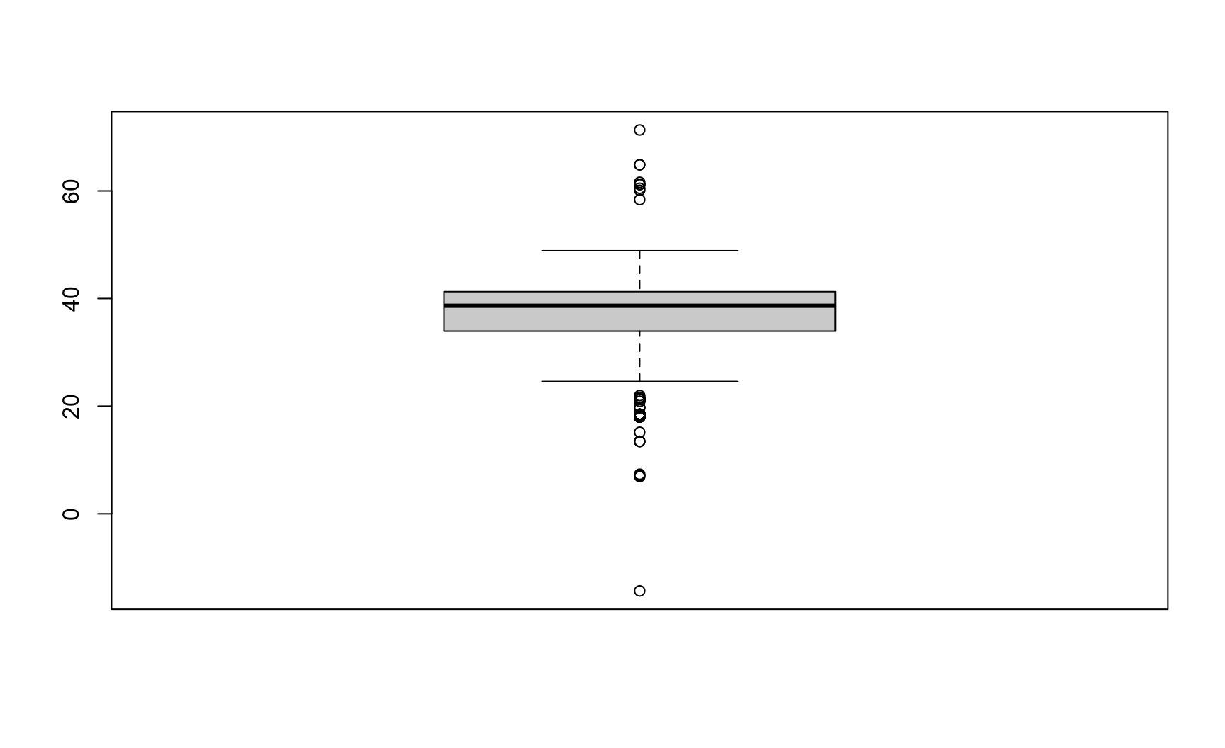
 -14.32   33.93   38.66   37.31   41.28   71.32

Do the minimum and maximum values make sense?
- E.g., a latitude outside of \([-90, 90]\) would be invalid.
A quick plot can also help spot outliers visually:

boxplot(universities$LATITUDE)

Check ranges by groups

Some ranges only make sense within a group — combine group_by() and summarise() to check them.

universities |>
  group_by(STABBR) |>
  summarise(
    min_lat = min(LATITUDE, na.rm = TRUE),
    max_lat = max(LATITUDE, na.rm = TRUE)
  )

# A tibble: 59 × 3
   STABBR min_lat max_lat
   <chr>    <dbl>   <dbl>
 1 AK        58.4    71.3
 2 AL        30.3    34.9
 3 AR        33.2    36.4
 4 AS       -14.3   -14.3
 5 AZ        31.6    36.3
 6 CA        32.6    41.4
 7 CO        37.2    40.6
 8 CT        41.1    42.0
 9 DC        38.9    38.9
10 DE        38.5    39.8
# ℹ 49 more rows

Checking variable types

Each variable should have the type you expect (e.g., a state code should be a character, a coordinate should be numeric).

# Check the type of a single variable
is.numeric(universities$LATITUDE)

[1] TRUE

is.character(universities$STABBR)

[1] TRUE

# Check the type of every column at once
sapply(universities, class)

     UNITID      INSTNM      IALIAS        ADDR        CITY      STABBR 
  "numeric" "character" "character" "character" "character" "character" 
        ZIP        FIPS      OBEREG       CHFNM    CHFTITLE     GENTELE 
"character"   "numeric"   "numeric" "character" "character"   "numeric" 
        EIN        DUNS       OPEID     OPEFLAG     WEBADDR    ADMINURL 
"character" "character" "character"   "numeric" "character" "character" 
    FAIDURL     APPLURL    NPRICURL      VETURL      ATHURL     DISAURL 
"character" "character" "character" "character" "character" "character" 
     SECTOR     ICLEVEL     CONTROL     HLOFFER     UGOFFER     GROFFER 
  "numeric"   "numeric"   "numeric"   "numeric"   "numeric"   "numeric" 
   HDEGOFR1    DEGGRANT        HBCU    HOSPITAL     MEDICAL      TRIBAL 
  "numeric"   "numeric"   "numeric"   "numeric"   "numeric"   "numeric" 
     LOCALE    OPENPUBL         ACT       NEWID     DEATHYR    CLOSEDAT 
  "numeric"   "numeric" "character"   "numeric"   "numeric" "character" 
   CYACTIVE     POSTSEC     PSEFLAG    PSET4FLG      RPTMTH     INSTCAT 
  "numeric"   "numeric"   "numeric"   "numeric"   "numeric"   "numeric" 
   C18BASIC     C18IPUG    C18IPGRD    C18UGPRF    C18ENPRF    C18SZSET 
  "numeric"   "numeric"   "numeric"   "numeric"   "numeric"   "numeric" 
   C15BASIC     CCBASIC    CARNEGIE    LANDGRNT    INSTSIZE    F1SYSTYP 
  "numeric"   "numeric"   "numeric"   "numeric"   "numeric"   "numeric" 
   F1SYSNAM    F1SYSCOD        CBSA    CBSATYPE         CSA       NECTA 
"character"   "numeric"   "numeric"   "numeric"   "numeric"   "numeric" 
   COUNTYCD    COUNTYNM    CNGDSTCD    LONGITUD    LATITUDE     DFRCGID 
  "numeric" "character"   "numeric"   "numeric"   "numeric"   "numeric" 
   DFRCUSCG 
  "numeric"

Checking variable types

is.numeric(), is.character(), is.logical(), is.factor(): each returns TRUE/FALSE.
sapply(..., class) applies class() to every column, giving you a full overview in one instruction.

Tip If a variable that should be numeric shows up as character, this is often a sign of a stray non-numeric value (e.g., "n/a" or a typo) somewhere in the column.

Exercise

Using the universities dataset, write a pipeline that:

Creates a new column sector_clean, equal to NA when SECTOR == 99, and equal to SECTOR otherwise.
Groups the institutions by sector_clean.
Computes, for each group, the number of institutions and their average latitude (LATITUDE).
Sorts the result so that the group with the lowest average latitude appears first.

Solution

universities |>
    mutate(
        sector_clean = ifelse(SECTOR == 99, NA, SECTOR)
    ) |>
    group_by(sector_clean) |>
    summarise(
        n_institutions = n(),
        avg_latitude = mean(LATITUDE, na.rm = TRUE)
    ) |>
    arrange(avg_latitude)

mutate(): recodes the placeholder value 99 as a genuine missing value (NA), so it doesn’t get treated as a real sector.
group_by(): splits the data by sector_clean (institutions with a missing sector form their own NA group).
summarise(): computes one row per sector, with n() for the count and mean(..., na.rm = TRUE) for the average latitude.
arrange(): sorts sectors from lowest to highest average latitude (i.e., from south to north).

Joining data

Joining is the mechanism which connects many datasets that are inter-related.
Whenever the data we need are distributed across several different sources, we need to combine them together to implement the data analysis.
Joining datasets requires identifying common key variables to perform the combination.

The `dplyr` package

We are going to use the {dplyr} package to join datasets.

install.packages("dplyr")
library(dplyr)

Four types of join

left_join()
right_join()
inner_join()
full_join()

See the 🌐 cheat sheet from dplyr.

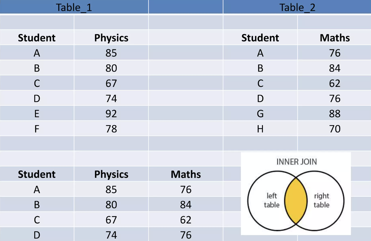
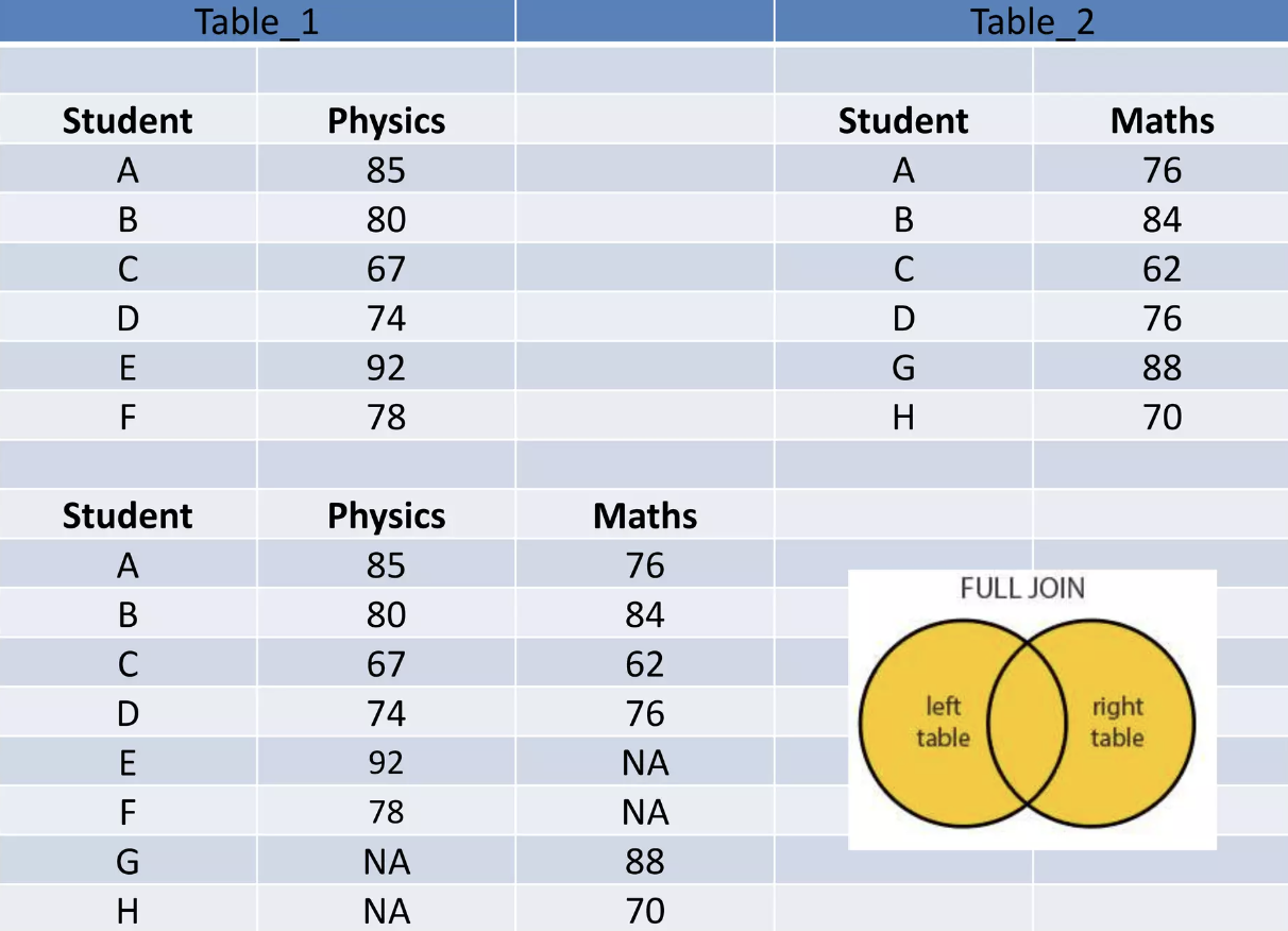
Example

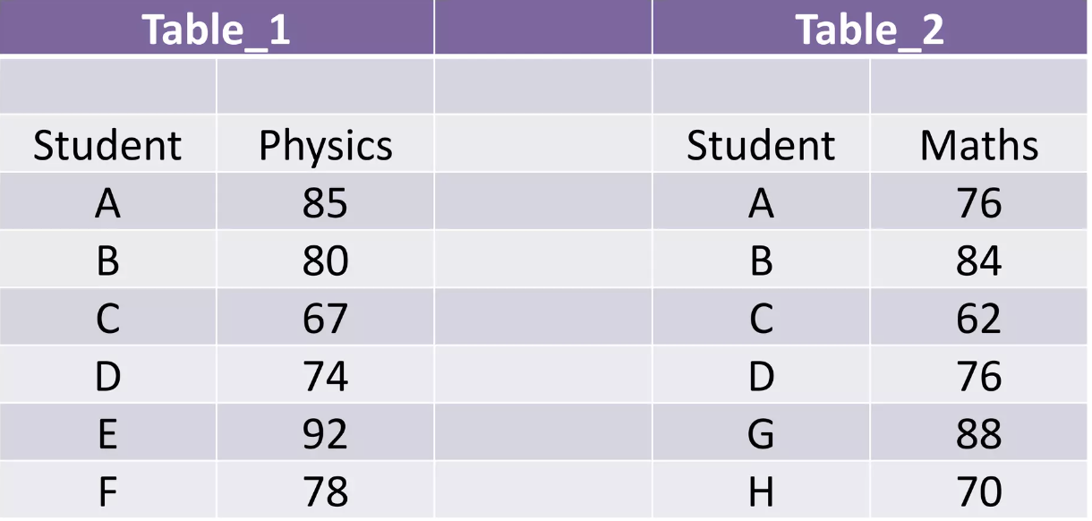
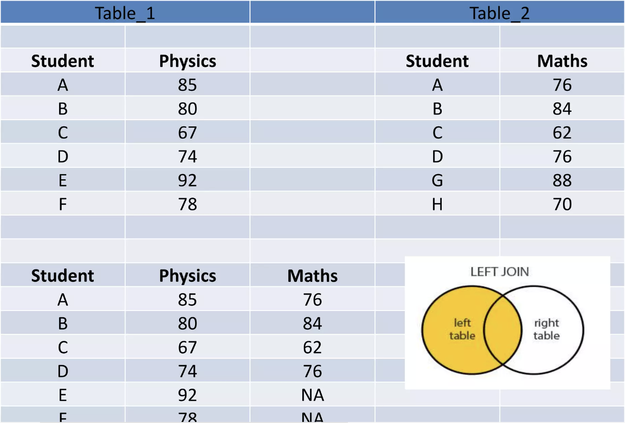
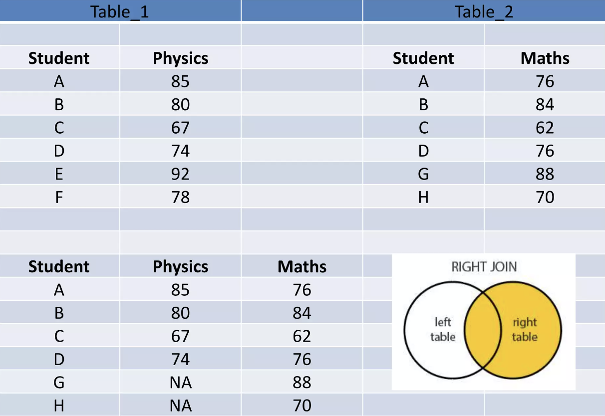
Let us consider a few examples to join these two tables.

These tables in `R`

library(dplyr)
physics_class <- tribble(
  ~Student, ~Physics,
  "A", 85,
  "B", 80,
  "C", 67,
  "D", 74,
  "E", 92,
  "F", 78,
)

math_class <- tribble(
  ~Student, ~Maths,
  "A", 76,
  "B", 84,
  "C", 62,
  "D", 76,
  "G", 88,
  "H", 70,
)

Requirements

To join datasets, we first need to identify a common key/identifier across datasets.
We then need to harmonize this common identifier across datasets (same format, same writing rules etc.).
Question: what could be the common identifier in this example?
Question: is the identifier harmonized across datasets?

`left_join()`

`right_join()`

`inner_join()`

`full_join()`

Exercise: Testing our hypothesis

Let us go back to the hypothesis from the beginning of this session:

Is the presence of a university in the county of residence of a given individual positively associated with the probability that this individual attends university?

Using universities and survey, write a pipeline that answers this question. You will need to:

Harmonize the county and state names so they match across the two datasets (careful with upper/lower case).
In survey, create a binary variable attend_university, equal to 1 if the individual completed more than 12 years of education (educ), 0 otherwise.
In universities, count the number of institutions per county (COUNTYNM) and state (STABBR).
Join this count onto survey, matching on county and state.
Create a binary variable indicating whether the individual’s county has at least one university.
Compare the proportion of individuals attending university, depending on whether their county has a university or not.

Hint str_to_upper() (from {stringr}) is useful to harmonize text casing before joining two datasets on a character key.

Solution

universities <- universities |> 
  mutate(
    COUNTYNM = str_to_upper(COUNTYNM)
  )

survey <- survey |> 
  mutate(
    attend_university = as.integer(educ > 12),
    state = str_to_upper(state)
  )

tb_n_univ_counties <- universities |> 
  count(COUNTYNM, STABBR, name = "n_univ_county")

survey_univ <- survey |> 
  left_join(
    tb_n_univ_counties,
    by = c("county" = "COUNTYNM", "state" = "STABBR")
  )

survey_univ |> 
  mutate(
    univ_county = !is.na(n_univ_county)
  ) |> 
  count(univ_county, attend_university) |> 
  group_by(univ_county) |> 
  mutate(prop = n / sum(n))

# A tibble: 4 × 4
# Groups:   univ_county [2]
  univ_county attend_university     n  prop
  <lgl>                   <int> <int> <dbl>
1 FALSE                       0  1453 0.496
2 FALSE                       1  1478 0.504
3 TRUE                        0    36 0.456
4 TRUE                        1    43 0.544

str_to_upper(): harmonizes the casing of county/state names in both datasets, so the join key matches exactly.
mutate(attend_university = ...): recodes years of education into a simple binary outcome.
count(COUNTYNM, STABBR, name = "n_univ_county"): counts institutions per county, renaming the result column directly.
left_join(): attaches the university count to each individual, based on their county and state of residence.
!is.na(n_univ_county): individuals whose county has no matching row in tb_n_univ_counties get NA, meaning no university in their county.
group_by(univ_county) |> mutate(prop = n / sum(n)): computes the proportion attending university, separately for individuals with and without a university in their county — this is the comparison that answers our hypothesis.

Exercises

Practice with the first tutorial!

You are expected to complete the exercises before the next session.

Introduction to programming for data analysis

Disclaimer

The 4 steps in any data analysis

Finding data

How can we find data?

A few advices from Alex the Analyst

Primary vs Secondary data

Description and Aim of the Session

Outline of the session

Finding data

Data strategy

Set Your RStudio Project

Exercise

Solution: Link to the Desired Dataset

Coding Preamble

What are functions? Libraries? and Loops?

What is a Function in R?

Key Components of a Function

Syntax

Example

Exercise

What is a Library in R?

Key Features of Libraries

Using Libraries in R

What is a Loop in R?

Types of Loops in R

for Loop Syntax and Example

while Loop Syntax and Example

Exercise

Importing data

Manage the Working Directory

Importing data

Import text files

Import text files: variants of read.table()

Export text files

Save/Load R objects

Exercise: Import

Solution: Import

What is a Clean Dataset?

Data are ready

Six Data quality indicators

Analyzable

Analyzable

Analyzable

Exercise

Solution

Interpretable

Exercise

Solution

Complete

Exercise

Solution

Valid

Exercise

Solution

Accurate

Exercise

Solution

Consistent

Exercise

Solution

Recap: Data validation

Standard Data Cleaning Checklist

Data Preparation with R

Working with the HD2018 dataset

A Glimpse at the Dataset

Core Syntax of dplyr

The Pipe Operator (|> or %>%)

The Data Refining Pipeline

Why Using The Data Refining Pipeline?

select()

mutate()

summarise()

group_by()

count()

Dataset dimensions

Missing values

Duplicate cases

arrange()

Counting to check completeness

What is a Function in `R`?

What is a Library in `R`?

Core Syntax of `dplyr`

The Pipe Operator (`|>` or `%>%`)

`select()`

`mutate()`

`summarise()`

`group_by()`

`count()`

`arrange()`

The `dplyr` package

These tables in `R`

`left_join()`

`right_join()`

`inner_join()`

`full_join()`