Course homepage

Introduction to programming for data analysis

Session 1 — Data Management

AMSE, Aix Marseille University

AMSE, Aix Marseille University

AMSE, Aix Marseille University

Disclaimer

  • The slides were adapted from those of Pierre Michel and Morgan Raux, both researchers at AMSE, who kindly shared their work.

  • This slide deck was made with Quarto and reveal.js, it is translated by Claude Sonnet 5 from a LaTex presentation previously made with beamer.

Introduction

Instructor

  • Ewen Gallic
  • Aix-Marseille School of Economics
  • Maître de Conférences (Assistant Prof.) in Economics
  • Research interests: data science, algorithmic fairness, environmental economics
  • Contact: ewen.gallic@univ-amu.fr
  • Office: 1-04, Îlot Bernard-du-Bois, Marseille

Course organization

  • Duration: 4 sessions (4 × 3 hours)
  • Introduction to programming for data analysis
  • Focus on the R language
  • Main objective: basic knowledge of R + tips to learn autonomously

What is NOT in the course

Warning This course does not cover all regression techniques!

  • It mostly focuses on the basic tools for importing, cleaning and exploring data.

Objectives

  • Introduction to the good practices to start an empirical research project
  • By the end of the course, you should be able to import data and conduct the first steps of an empirical analysis

Outline of the course

  1. Data management: file paths / .R scripts
  2. Cleaning data, combining different data sources (data “wrangling”)
  3. Producing summary statistics and data visualization
  4. Implementing first tests and regressions

Main reference for the course

Wickham, H., Cetinkaya-Rundel, M., Grolemund, G. 2023. R for Data Science: Import, Tidy, Transform, Visualize, and Model Data. O’Reilly Media, Incorporated.
🌐 https://r4ds.hadley.nz/

What can I get from this course?

This course will (hopefully) be useful for:

  • the continuation of your studies
  • but also for your professional career, especially for students who want to:
    • do a PhD and academic research
    • work in public institution
    • work in the private sector

This course will particularly be useful for those who want to work as economist, analyst, data scientist or consultant. Nowadays, a lot goes through data analysis.

Evaluation

  • The examination will be a take-home assignment
  • You will have to conduct a small data project
  • You will have to find data and conduct an empirical analysis to answer a questionnaire (available on Ametice)
  • You will be guided during classes
  • If you pay attention during classes, it will not ask you much extra work

Questions?

The R programming language and programming software

General information on R

  • R (1995, AT&T Bell Laboratories) is a software for statistical analysis and graphics, it is a clone of S-PLUS, mainly written in C language.
  • R is free software, distributed freely under the terms of GNU Public Licence of the Free Software Foundation (FSF). The development and distribution are ensured by several statisticians (R Development Core Team). It is compatible with all platforms.
  • Files and instructions for installing R, tutorials and updates are available from the CRAN (Comprehensive R Archive Network).

Downloading and installing R

  • Download R:
    🌐 https://cloud.r-project.org/
  • Install R on your computer
  • R is a programming language, it consists of a series of tools (packages)
  • After installing R, your computer can load these packages and let you use their content (functions, datasets, help pages)

Downloading and installing RStudio

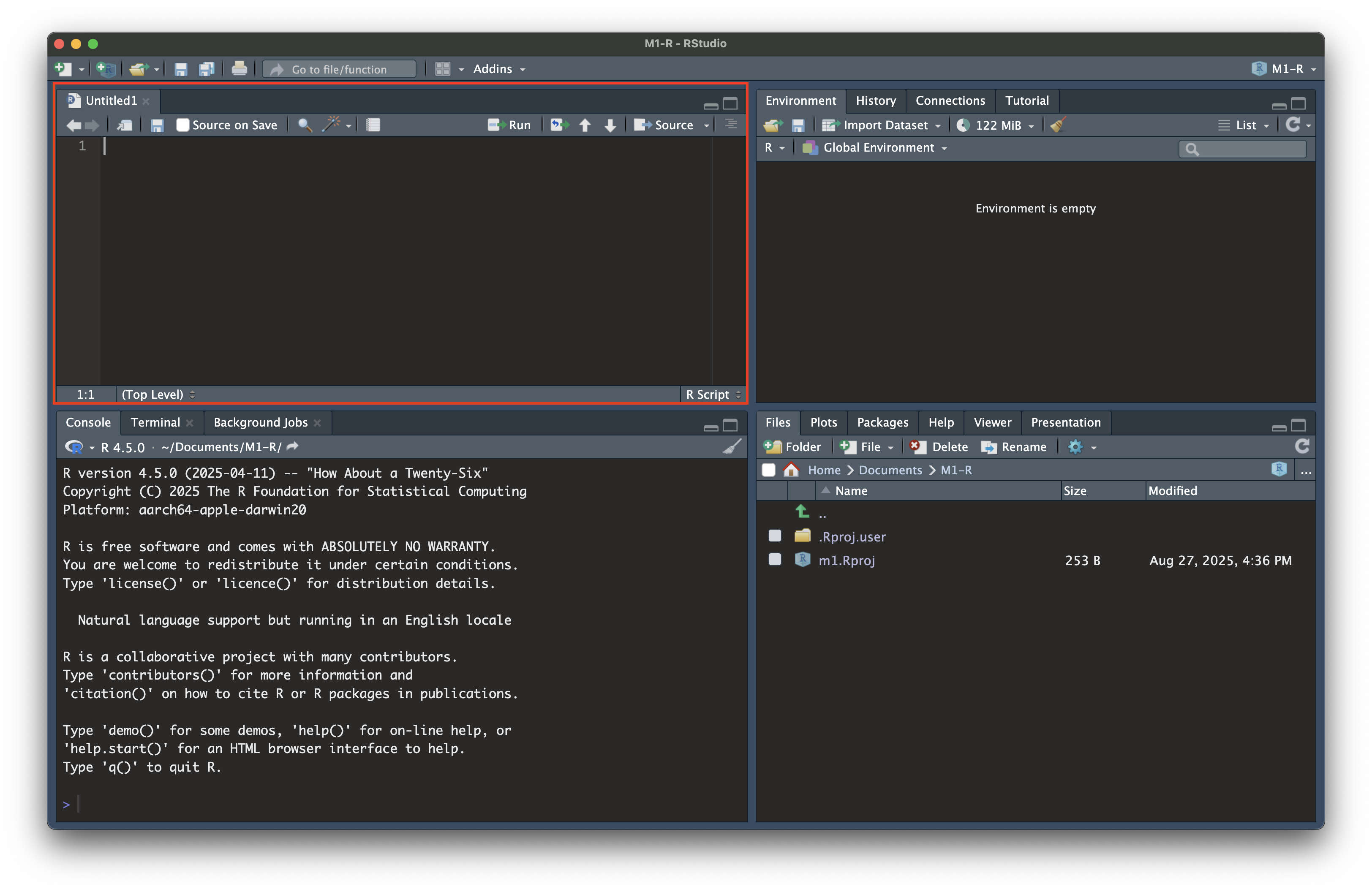
Interface presentation: .R Script

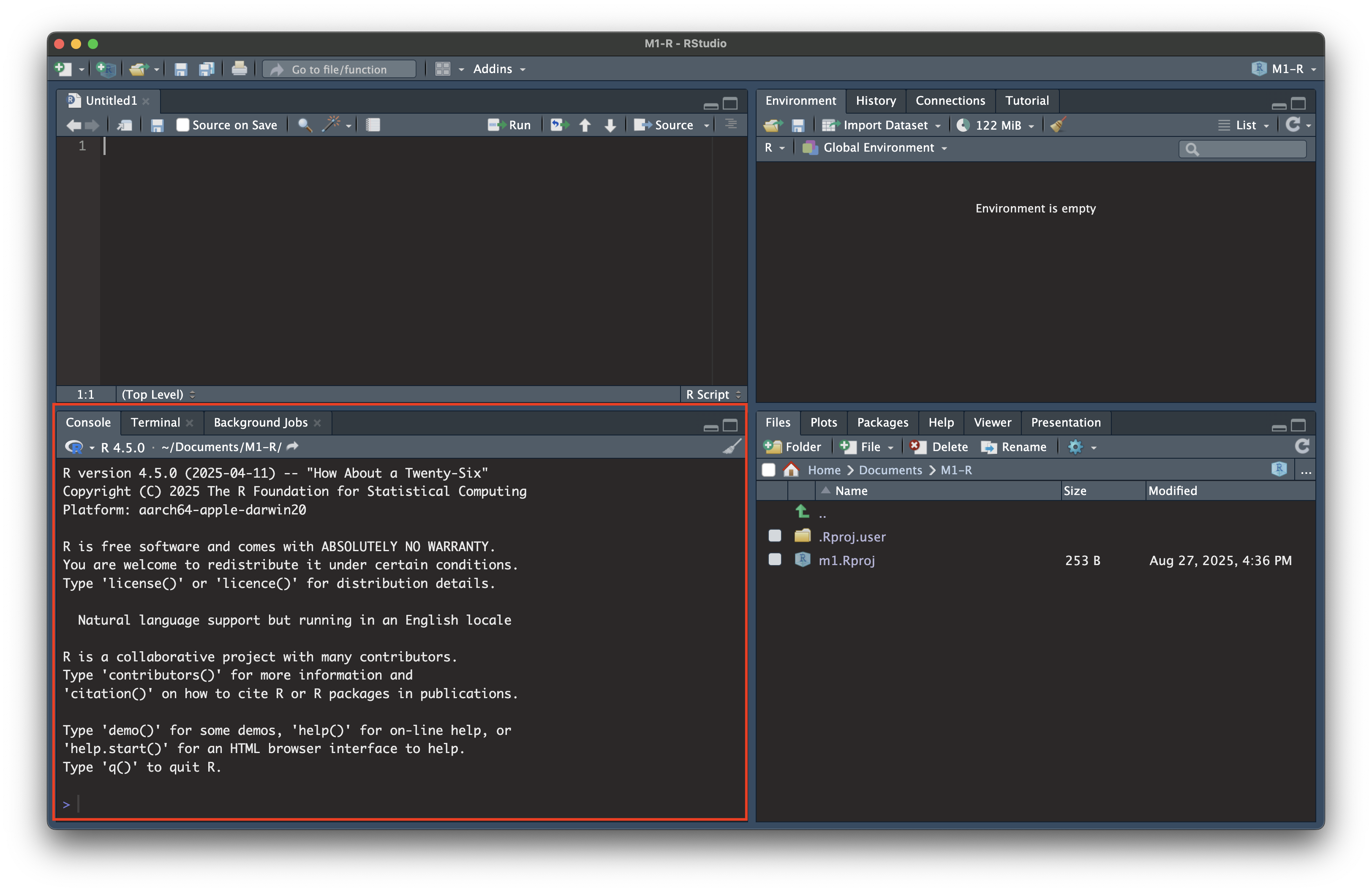
Interface presentation: the console

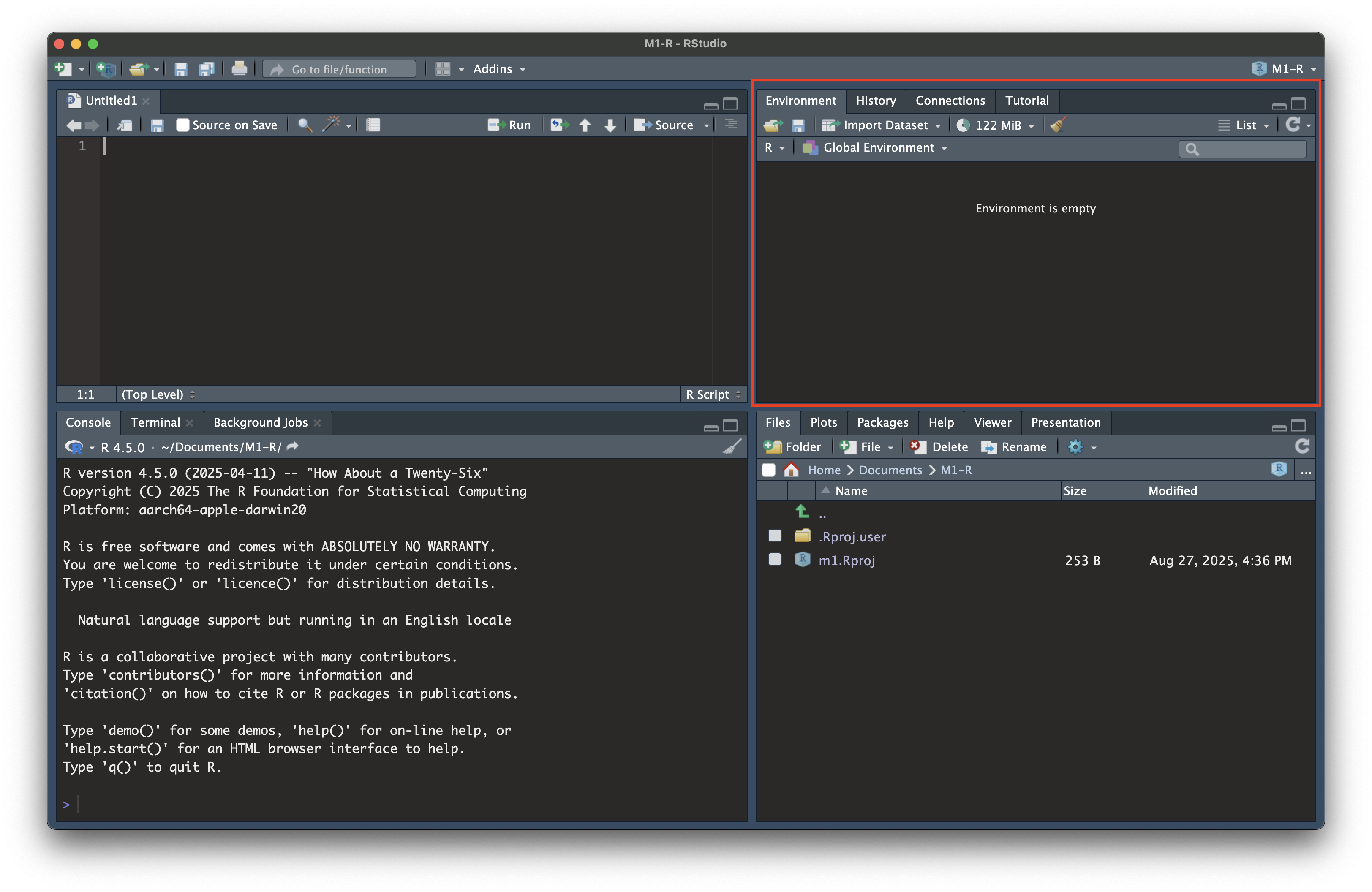
Interface presentation: where are the data?

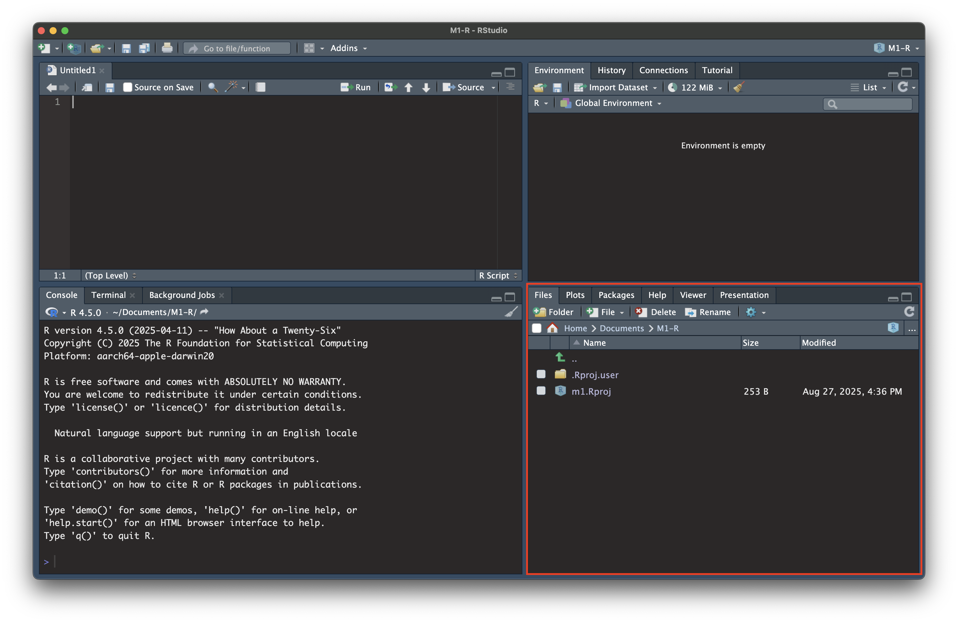
Interface presentation: file browser

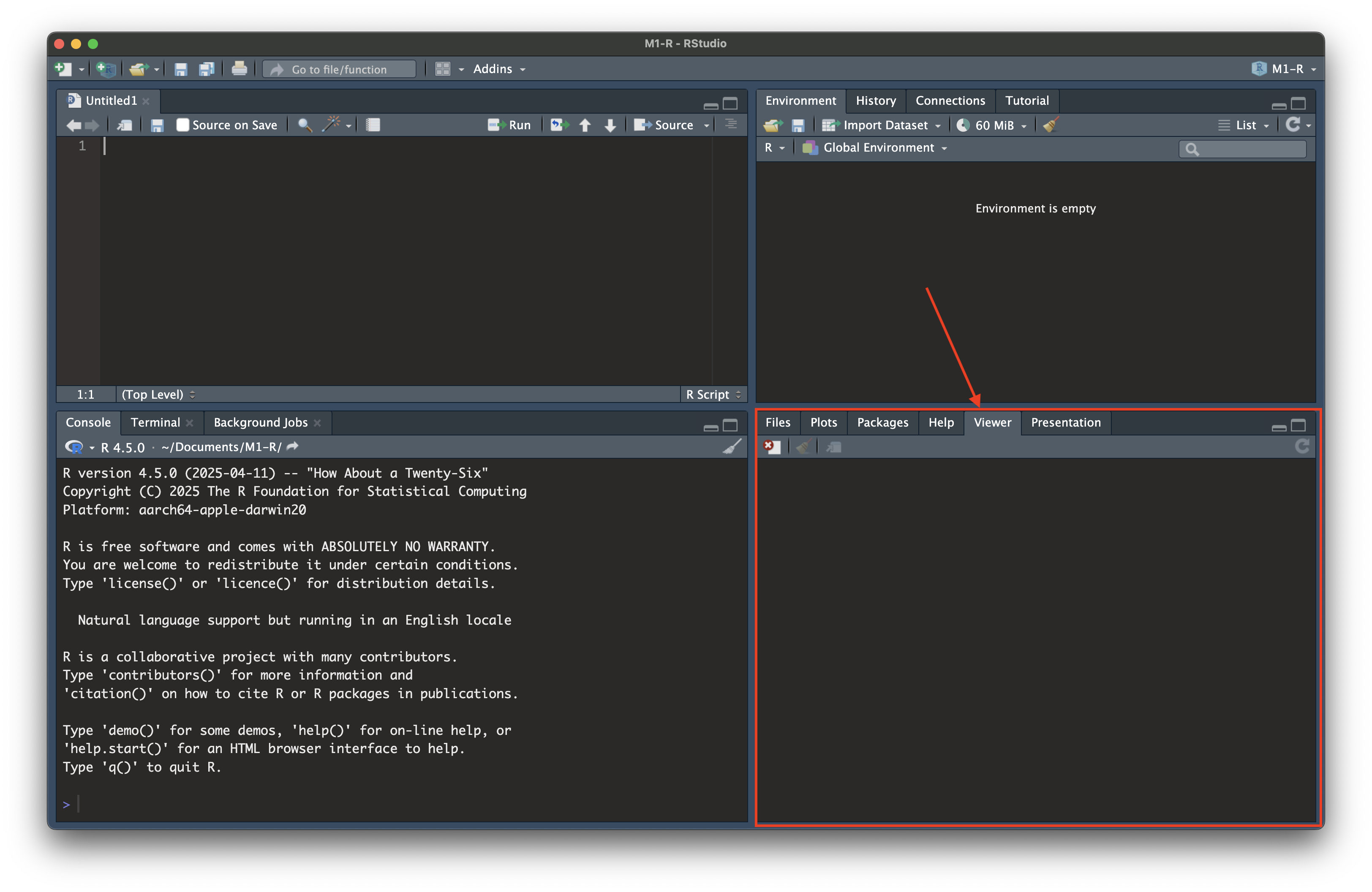
Interface presentation: viz viewer

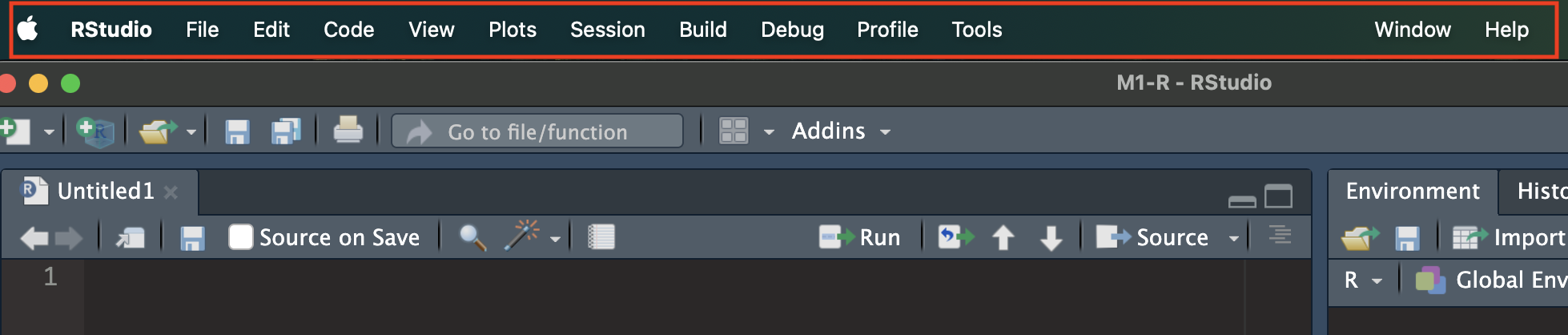
Interface presentation: the menu

General information

The R programming language is:

  1. interpreted: the available functions are located in a library, organized in packages containing functions, operators and datasets.
  2. object-oriented: variables, data, results in a R session are stored as objects in memory in the workspace.

The R console: your first calculator

  • Before writing any script, open the console (bottom-left pane in RStudio) and try typing some math directly.
  • R evaluates whatever you type and prints the result right away, exactly like a calculator.
1 + 1
10 / 3
2^10
sqrt(81)
  • Try it yourself: type a small calculation directly into the console and press Enter.

Storing values: variables and assignment

  • Typing a calculation in the console is useful, but the result disappears once you move on.
  • To keep a value, we store it in a variable, using the assignment operator <-.
x <- 5      # x now contains the value 5
y <- 3
x + y       # uses the stored values
  • Read x <- 5 as “x gets the value 5”.
  • Once created, a variable appears in the Environment tab of RStudio, and can be reused in later lines of code.

Tip = also works as an assignment operator in R, but <- is the convention used by the R community: stick to it!

Comments: leaving notes in your code

  • A comment starts with #. Everything after # on that line is ignored by R. It is there for humans, not for the computer.
  • Comments explain why you wrote a piece of code, so that you (or someone else) can understand it later.
# Compute the average of three exam scores
score_1 <- 12
score_2 <- 15
score_3 <- 9

average_score <- (score_1 + score_2 + score_3) / 3 # simple arithmetic mean
print(average_score)

Get into the habit early Add comments as you write your code, not afterward. A script without comments is much harder to read again in two weeks, even for its own author.

Data types in R

Every piece of data in R has a type. The three most common ones you will encounter are:

  • numeric: numbers, with or without decimals (2, 3.14, -7).
  • character: text, always written between quotes ("Marseille", "A").
  • logical: only three possible values, TRUE, FALSE or NA_logical.
age <- 25            # numeric
city <- "Marseille"  # character
is_student <- TRUE   # logical

Checking the type of a variable

  • The function class() tells you the type of any object in R.
class(age)         # "numeric"
class(city)        # "character"
class(is_student)  # "logical"
  • This is very useful when debugging: many errors come from a variable having a different type than what you expected.

Tip Logical values behave like numbers in disguise: TRUE equals 1 and FALSE equals 0. Try TRUE + TRUE in your console!

Vectors: grouping values together

  • A vector is an ordered collection of values of the same type. It is built with the function c() (for “combine”).
ages <- c(25, 31, 42, 19)
cities <- c("Marseille", "Paris", "Lyon")
is_passing <- c(TRUE, FALSE, TRUE, TRUE)
  • A single number, like age <- 25 earlier, is technically just a vector of length 1.
  • Vectors are the building block of almost everything else in R.

Working with vectors

  • Arithmetic operations apply to a whole vector at once (this is called vectorization).
ages <- c(25, 31, 42, 19)
ages + 1        # adds 1 to every element
mean(ages)      # average of the vector
length(ages)    # number of elements
  • Use square brackets [ ] to access a specific element by its position.
ages[1]   # first element: 25
ages[3]   # third element: 42
  • To get multiple elements by their positions, use a vector:
ages[c(1,3)]   # first and third elements: 25 and 42

Matrices: vectors in two dimensions

  • A matrix is a rectangular collection of values of the same type, arranged in rows and columns.
m <- matrix(
    c(1, 2, 3, 4, 5, 6),
    nrow = 2, ncol = 3
)
print(m)
  • Use two indices in square brackets, [row, column], to access a specific element.
m[1, 2]  # element in row 1, column 2
m[2, ]   # entire second row

Data frames: tables of data

  • A data frame is the structure you will use the most in this course: it is a table, where each column can have its own type (numeric, character, logical…).
  • It is built with the function data.frame().
students <- data.frame(
    name = c("Alice", "Bob", "Chloé"),
    age = c(21, 23, 22),
    is_erasmus = c(TRUE, FALSE, TRUE)
)
print(students)
  • Each row is an observation, each column is a variable.

Basic structures: summary

Structure Dimensions Types allowed Built with
Vector 1D one type c()
Matrix 2D one type matrix()
Data frame 2D one type per column data.frame()
  • Data frames are the closest to what you already know as a “spreadsheet” or a “dataset”.
  • Most of this course will consist of manipulating data frames.

Exercise

  1. Create a variable budget containing the number 1500. Add a comment above the line explaining what it stores.
  2. Create a variable name containing your first name, and a variable is_registered set to TRUE.
  3. Use class() to check the type of each of the three variables you just created.
  4. Create a vector weekly_expenses containing four numbers of your choice.
  5. Compute the total and the average of weekly_expenses, using sum() and mean().
  6. Build a small data frame budget_tracker with two columns: item (a character vector with 3 expense categories, e.g. "Rent", "Food", "Transport") and amount (a numeric vector with 3 corresponding amounts).
  7. Print budget_tracker, then check the class of each of its two columns.

Solution

# budget: how much money is available this month (numeric)
budget <- 1500

# name: my first name (character)
name <- "Camille"

# is_registered: whether I am registered for the course (logical)
is_registered <- TRUE

class(budget)          # "numeric"
class(name)            # "character"
class(is_registered)   # "logical"

# A vector of 4 weekly expenses
weekly_expenses <- c(120, 95, 60, 140)

sum(weekly_expenses)    # total expenses
mean(weekly_expenses)   # average weekly expense

# A small data frame tracking a few budget items
budget_tracker <- data.frame(
    item = c("Rent", "Food", "Transport"),
    amount = c(600, 250, 80)
)
print(budget_tracker)

class(budget_tracker$item)    # "character"
class(budget_tracker$amount)  # "numeric"

Sources to find help

  • The help pages of the R packages
  • Stackoverflow: generalist forum for coding help
  • Just google your question including “R” as a keyword in your search
  • Search on Youtube
  • Ask a generative AI chatbot (e.g., ChatGPT, Claude, Gemini)

A good help for coding: ChatGPT

  • Gen AI are incredibly useful to learn coding, especially in R (also true for Python)
  • You can just ask the bot how to code “task 1” or “task 2” in R
  • For simple tasks, you don’t even need to know anything about R
  • However, ChatGPT is not magic. Answers are sometimes irrelevant and you need to understand the R language to interpret the error messages you can face and adapt the code accordingly
  • Let us take 5 minutes to create an OpenAI account to use ChatGPT.
    🌐 https://chatgpt.com/

Concepts

What is a data analysis?

  • Doing a data analysis can be viewed as:
    • putting together data, preparing them,
    • computing statistics (descriptive, clustering, PCA, …), comparing,
    • extract information/knowledge and communicate them (text, figures, visualization)
  • We often create groups of observations
  • These groups might be defined by country, city, company, university, time period, ethnicity, hair color, …
  • Let us consider a few examples

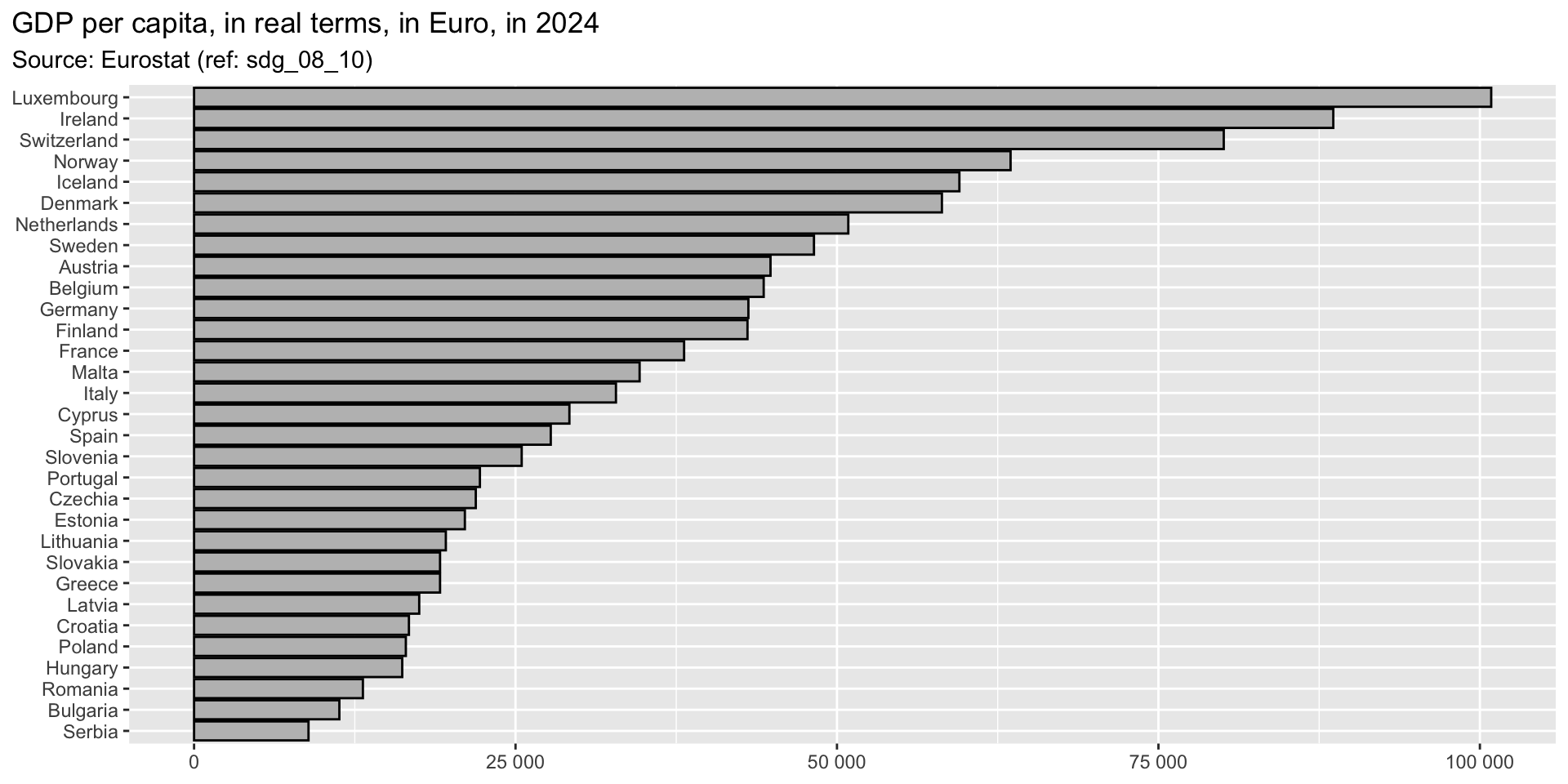
Example 1: comparison across countries

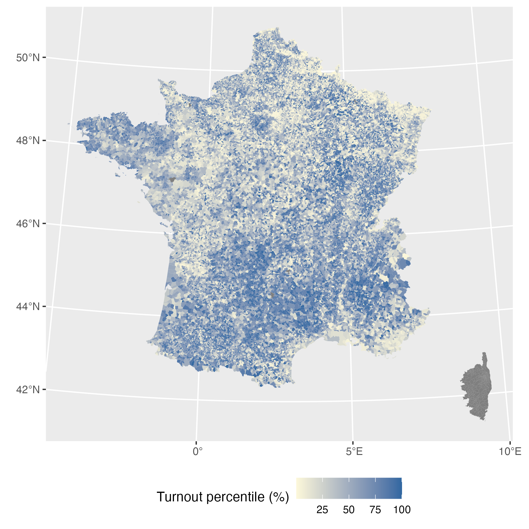
Example 2: comparison across cities

Comparing voter turnout between French cities for the 2024 parliamentary elections.

Source: data.gouv.fr
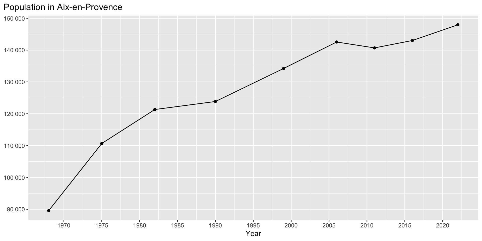
Example 3: comparison over time

Comparing the number of inhabitants in Aix-en-Provence over the years

Data analyses are increasingly present in our lives

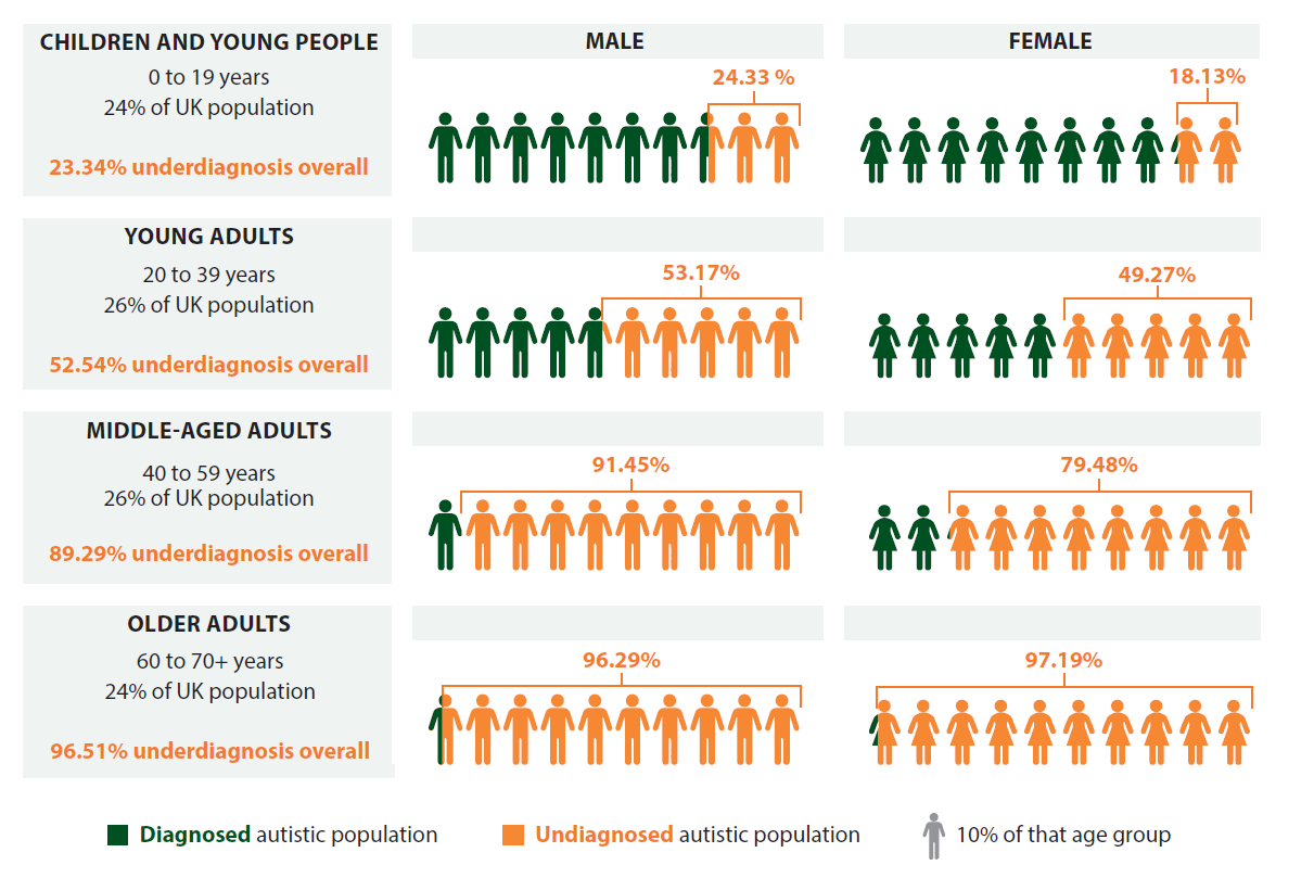
Data analyses create “knowledge” out of data.

Over 89 per cent of autistic adults aged 40+ are undiagnosed.

Source: Annual Review of Developmental Psychology1, King’s College London
Data analyses are increasingly present in our lives

Data analyses are also used to take decisions.
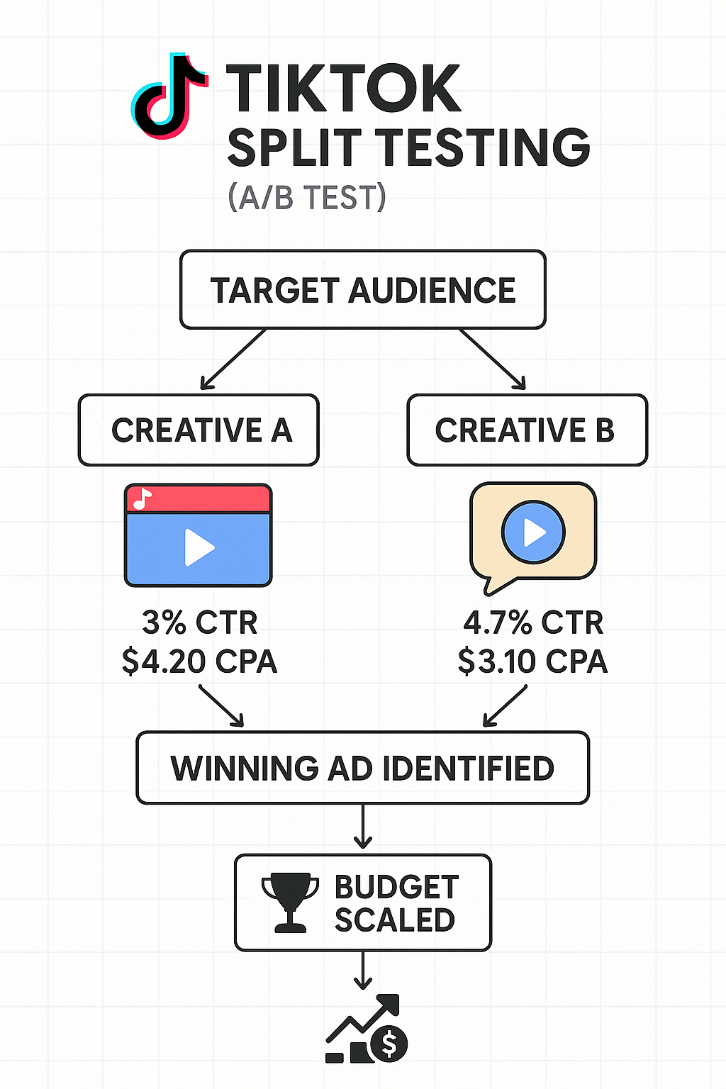
Source: generated by ChatGPT-5

Who are doing data analyses?

  • Research institutions (universities, research centers, etc.)
  • Private companies (start-ups, big corporations, etc.)
  • Public institutions (ministries, OECD, IMF, etc.)

Data analysis is one of the most important skills you can provide at the beginning of your “economist” career.

What are the data?

  • Definition: we can call data anything that can be measured AND structured into a dataset
  • Where do they come from?
    • Survey Data: responses collected from a group of individuals using a structured questionnaire to gather information on various topics.
    • Sensor Data: continuous measurements recorded by sensors, such as temperature, humidity, or motion.
    • Transaction Data: records of individual transactions in a business, including details like date, time, amount, and items purchased.
    • Administrative data: data collected and maintained by organizations or institutions as part of their routine operations and administrative processes.

What is a dataset?

Definition: A dataset is a collection of data, typically organized in a structured format. It consists of multiple observations (rows), each described by one or more variables (columns).

ID Name Age Gender Income
1 Alice 30 Female 55000
2 Bob 45 Male 60000
3 Charlie 25 Male 50000
  • Each row (ID 1 to 3) is an observation. It represents a different individual.
  • The columns (ID, Name, Age, Gender, Income) are the variables. They represent different characteristics of the individuals.

What are the different types of data in economics?

In economics, we mostly find the following data structures:

  1. Cross-sectional data: data collected at a single point in time across multiple units (e.g., individuals, households, firms, countries, regions, …)
  2. Panel data: data that follows multiple units (e.g., individuals, firms, countries) over two or more time periods.
    • You may also have heard the term longitudinal data to refer to panel data.

Cross section data example

Id Name University Earnings
1 Alex Harvard 120K
2 Sarah Yale 100K
3 Marie NYU 110K

In this example, the unit of observation is (individual).

Panel data example

Id Name University Application Earnings
1 Alex Harvard Harvard 120K
1 Alex Harvard Princeton 120K
2 Sarah Yale Yale 100K
2 Sarah Yale Stanford 100K
2 Sarah Yale UC Berkeley 100K
3 Marie Princeton Princeton 110K
3 Marie Princeton Harvard 110K

In this example, the unit of observation is (individual, application).

Panel data example 2

Id Name Univ. Appl. 1 Appl. 2 Appl. 3 Earnings Year
1 Alex Harvard Harvard Princeton . 120K 2010
1 Alex Harvard Harvard Princeton . 130K 2011
1 Alex Harvard Harvard Princeton . 150K 2012
2 Sarah Yale Yale Stanford UC Berkeley 100K 2010
2 Sarah Yale Yale Stanford UC Berkeley 100K 2011
2 Sarah Yale Yale Stanford UC Berkeley 105K 2012
3 Marie Princeton Princeton Harvard . 110K 2010
3 Marie Princeton Princeton Harvard . 90K 2011
3 Marie Princeton Princeton Harvard . 110K 2012

In this example, the unit of observation is (individual, year).

What do we compare in a data analysis?

Two key concepts to properly understand the comparisons we make in data analyses:

  • Unit of observation
  • Sources of variations

Unit of observation

  • Unit of observation: the entity that each row of your data represents. It could be an individual, a household, a company, a country, a year, an event, or any other entity depending on the context of your study.
  • If each row in your dataset represents a person, then the unit of observation is an individual.
    • Example: A dataset containing survey responses from 1,000 people, where each row represents one person’s responses.
  • If each row represents a company, then the unit of observation is a company.
    • Example: A dataset with financial data for 100 companies.

Sources of variations

  • Implementing a data analysis boils down to making comparisons.
  • The comparisons we can do depend on the data we have.
  • Depending on the structure of the data, there are different types of comparisons we can make.
  • Depending on the comparison we are making, we can exploit different sources of variations.
  • Let us consider several examples to better understand.

Example 1: Survey among students

I have collected information among students with a google questionnaire on April 20, 2024.

What is the structure of my dataset?

  1. Cross-section dataset
  2. Panel dataset

Answer: Panel dataset

Example 1: Survey among students

What is the unit of observation in this dataset?

  1. A group of students
  2. A student in a given year
  3. A student

Answer: A student

Example 1: Survey among students

What comparisons can I make out of this dataset? (what are the sources of variations?)

  1. I can compare universities
  2. I can compare students with each other
  3. I can compare students over time

Answer: I can compare students with each other

Example 2: Payments list

Let us imagine we have access to the list of all payments made by the clients of one bank.

What is the structure of my dataset?

  1. Cross-section dataset
  2. Panel dataset

Answer: Panel dataset

Example 2: Payments list

What is the unit of observation in this dataset?

  1. A payment
  2. A customer of the bank
  3. A customer in a specific year

Answer: A payment

Example 2: Payments list

What comparisons can I make out of this dataset? (what are the sources of variations?)

  1. I can compare the payments made by different customers
  2. I can compare the payments made over time
  3. I can compare the payments made by one customer over time

All three are valid sources of variation here.

Identifying the right source of variations

  • There is often several sources of variations in one dataset.
  • To make accurate interpretation of the statistics we are going to produce, we need to understand what exactly are the variations we are exploiting.
  • In other words, we need to perfectly understand the comparisons we are making.

Good practices for data analyses

Why good coding practices are important?

  • Coding is a critical component of high-quality reproducible research (true for both academic and non-academic research).
  • Save time and energy: coding enables you to automate everything that can be done.
  • Coding also enables you to keep track of all steps you implemented to obtain a specific estimate.

Organizing folders

  • Over the life-cycle of a project, we accumulate files…
  • These originate from:
    • Getting raw data,
    • Writing programs to process the data,
    • Putting together data for analysis,
    • Generating tables, graphs and figures.
  • And, of course, there are several versions of all of the above.
  • All of these files should be sorted in folders.

My suggestion of folder structure

Root
  data
    raw
    tmp
    out
  functions
    utils.R
  scripts
    your-script-1.R
    your-script-2.R
  notebooks
    your-notebook-1.Rmd
    your-notebook-2.Rmd
  figs
  tables
  references
  README.md
  project.Rproj

  • Root is, here, your working directory: the default folder where your programs look for files to read, and where they save the files you create, unless you tell them otherwise.
    • It’s like the “home base” for your project. When you use a relative path (e.g., "data/raw/data.csv"), R looks for that file starting from the working directory.
    • You can always change it (setwd()), but best practice is to keep it at your project’s root folder.
    • Analogy with a GPS: “Go north two green lights” only makes sense if we know where you’re starting from.

Root folders — data/

Root
  data
    raw
    tmp
    out
  functions
    utils.R
  scripts
    your-script-1.R
    your-script-2.R
  notebooks
    your-notebook-1.Rmd
    your-notebook-2.Rmd
  figs
  tables
  references
  README.md
  project.Rproj

data: includes your data in folders:

  • raw: the raw data you have collected
  • tmp: temporary modified data you create along the process but will not include when/if you share your codes
  • out: final data files you will be using in the analysis

Root folders — functions/

Root
  data
    raw
    tmp
    out
  functions
    utils.R
  scripts
    your-script-1.R
    your-script-2.R
  notebooks
    your-notebook-1.Rmd
    your-notebook-2.Rmd
  figs
  tables
  references
  README.md
  project.Rproj

functions: folder containing the scripts with the functions you wrote.

The script files will be loaded in your analysis scripts, using the source() function.

Root folders — scripts/

Root
  data
    raw
    tmp
    out
  functions
    utils.R
  scripts
    your-script-1.R
    your-script-2.R
  notebooks
    your-notebook-1.Rmd
    your-notebook-2.Rmd
  figs
  tables
  references
  README.md
  project.Rproj

scripts: folder containing the scripts you write to prepare the data and to perform the analysis.

Root folders — notebooks/

Root
  data
    raw
    tmp
    out
  functions
    utils.R
  scripts
    your-script-1.R
    your-script-2.R
  notebooks
    your-notebook-1.Rmd
    your-notebook-2.Rmd
  figs
  tables
  references
  README.md
  project.Rproj

notebooks: your notebooks explaining step-by-step your methodology/codes.

Root folders — figs/ and tables/

Root
  data
    raw
    tmp
    out
  functions
    utils.R
  scripts
    your-script-1.R
    your-script-2.R
  notebooks
    your-notebook-1.Rmd
    your-notebook-2.Rmd
  figs
  tables
  references
  README.md
  project.Rproj

figs and tables: folders containing the exported figures and tables produced by your analysis.

Root folders — references/

Root
  data
    raw
    tmp
    out
  functions
    utils.R
  scripts
    your-script-1.R
    your-script-2.R
  notebooks
    your-notebook-1.Rmd
    your-notebook-2.Rmd
  figs
  tables
  references
  README.md
  project.Rproj

references: folder containing the PDF versions of the academic papers or documents from the grey literature used to perform your analysis.

Some conventions and recommendations

  • Never use spaces in folder or file names, to keep them machine readable.
    • Replace spaces with hyphens (-, best practice if you plan on sharing files on the Internet), or with underscores (_).
  • In your scripts, use comprehensive names for your variables, and try to make the names as short as possible.
    • Avoid calling variables a, aa, aaa, foo, bar, …
  • Add comments to your code at the same time as you write your scripts: while you may view this as losing time, it will not only help you return more easily to what you did, but it will also benefit other readers who may try to reuse your scripts.
  • Please read the following short guide made by people from the tidyverse community: https://style.tidyverse.org/

A few tips on file names

  • Use prefixes and suffixes in your script files names.
  • Having sequence numbers prefixed to script files helps sort them out and align them with the workflow, while suffixes track the version numbers.
  • Example:
    • 01-prepare-data-v4.R
    • 02-merge-v2.R
    • 03-summary-statistics-v11.R
    • 04-regressions-v15.R
  • Drawback: if you want to add an additional step, you’ll need to rename files in batches.
  • Move older files away from the main folders: create an old folder inside your scripts folder.
  • Apply the same naming conventions to graphs and tables.

Set Your RStudio Project

Root
  data
    raw
    tmp
    out
  functions
  scripts
  notebooks
  figs
  tables
  references
  project.Rproj

  1. Open RStudio

  2. Create a new project

    • FileNew Project...
    • Choose New Directory
    • Create a project named session-1
  3. Create the project structure

    In the R console, run:

dir.create("data")
dir.create("data/raw")
dir.create("data/tmp")
dir.create("data/out")
dir.create("functions")
dir.create("scripts")
dir.create("notebooks")
dir.create("figs")
dir.create("tables")
dir.create("references")

Setting up a project with RStudio

  • Now that we have created all the different folders from our architecture, we can create an .Rproj file.
  • RStudio is a coding environment for R.
  • We can use its graphical interface to import and save data from the ‘Environment’ tab.
    • If you do so, you’ll notice that the path to the data file is not relative to the working directory.
    • Instead of using the buttons, we will prefer the option to write ourselves the path to the data file and the import options.

What is a .R script?

  • A .R script is an ASCII (American Standard Code for Information Interchange) file which contains R instructions typed in plain text.
  • Compared to the console, the script allows you to keep track of instructions and to evaluate them in a specific order.
  • Open a new .R script from the graphic interface (or using the keyboard shortcut).
  • You can (re)open a .R script from the graphic interface or just by clicking on your .R script in the corresponding folder.

Start with a .R script

  • Our goal for now is to write an R code interacting with our different subfolders.
  • To do so, we define relative paths in a .R script.
  • Relative paths tell RStudio where to look for resources to interact with (either for opening, reading, writing, appending, closing, deleting, renaming).
  • See exercise 1 from the tutorial.

Good practices for .R scripts

  • Do not hesitate to skip lines for better readability.
  • On RStudio, in the script window, you can notice a vertical line at 80 characters from the left of the text area: do not write comments or code after that vertical line.
  • Use comments and annotations:
    • # identifies what is followed until the next line as a comment. Anything written after a # will be ignored by the interpreter.
  • Use different .R scripts for different tasks:
    • ./scripts/01-clean-data-v1.R
    • ./scripts/02-summary-stats-v1.R
    • ./scripts/03-regressions-v1.R

Application

Rules of the application/exam

In your exam, you will need to:

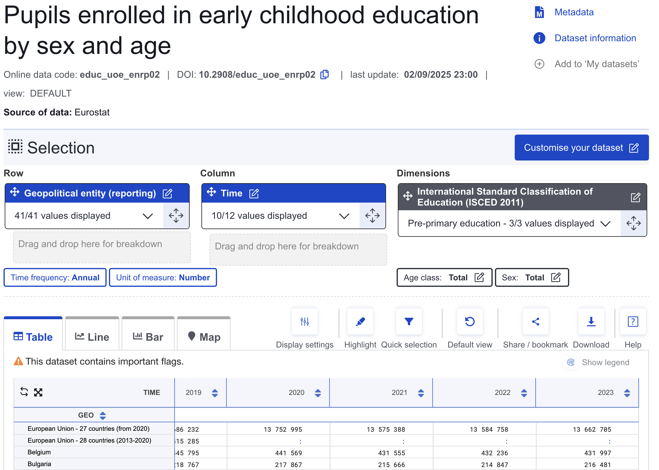
  • Download data from Eurostat.
  • Clean and assemble the different sources of data from Eurostat.
  • Draw summary statistics and save them in tables and graphs.
  • Run a basic regression.

Let us start by finding data on Eurostat!

Finding data on Eurostat

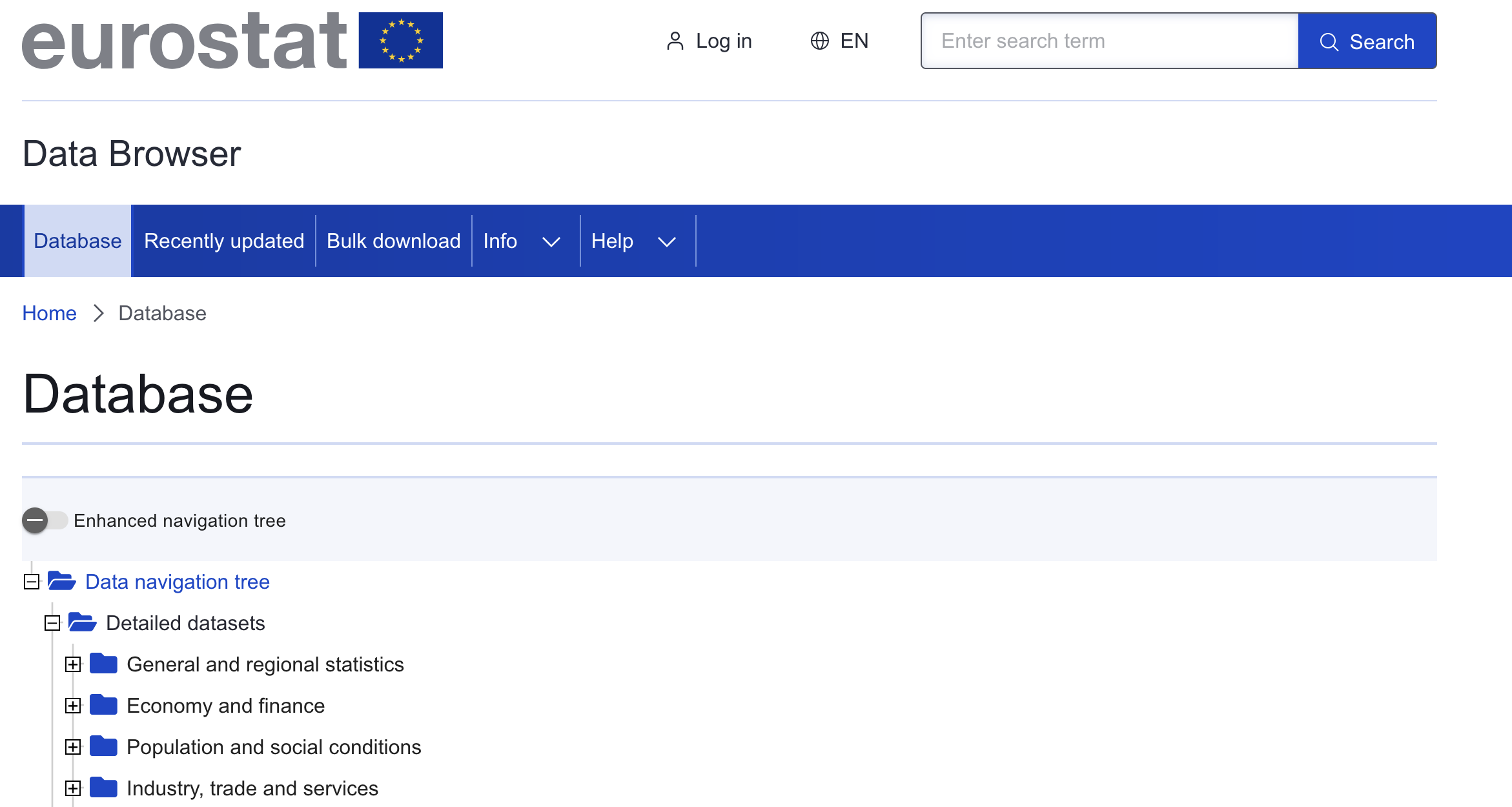
🌐 Eurostat data browser

Eurostat data browser

For your exam

  1. You must find and choose 2 dimensions (2 variables) in Eurostat data to explore in your analysis.
  2. You must download the data from Eurostat.
  3. You must then combine (match) the different files together.
  4. This will form your dataset to be used in your data analysis.
  5. You need to get the data for next week!