Maps with R
Rennes, 14 janvier 2015
Ewen Gallic
http://egallic.fr
Outline
- A (really) Short Introduction to R
- How to Manipulate Data
- The Basics of Graphics with ggplot2
- Maps
Some Useful References
- Anderson, S. (2012). A quick introduction to plyr.
- Charpentier, A. (2014). Computational actuarial science with R. Chapman and Hall.
- Gallic, E. (2015). Logiciel R et programmation.
- Goulet, V. (2014). Introduction à la programmation en R.
- Lafaye de Micheaux, P., Drouilhet, R., & Liquet, B. (2011). Le logiciel R : Maîtriser le langage - effectuer des analyses statistiques. Springer.
- Paradis, E. (2002). R pour les débutants.
- Wickham, H. (2009). ggplot2 : Elegant graphics for data analysis. Springer.
- Zuur, A., Ieno, E. N., & Meesters, E. (2009). A beginner’s guide to R. Springer.
A (Really) Rhort Introduction to R

What is R?
R is a free software environment for statistical computing and graphics. It compiles and runs on a wide variety of UNIX platforms, Windows and MacOS. (https://www.r-project.org/)
Language inspired by S, a programming language deveoloped in the 1970s by John Chambers, Douglas Bates, Rick Becker, Bill Cleveland, Trevor Hastie, Daryl Pregibon and Allan Wilks from the AT&T Bell Laboratories
R was created in the middle of the 1990s, by Ross Ihaka and Robert Gentleman from the University of Auckland
Distributed under the GNU General Public License
Developped and distributed by the R Development Core Team
Useful to manipulate data, realise statistical analysis, create graphics, ...
Working Environment
- R is an interpreted language
- There is no compilation
- One can either work directly on the console or on a script file
RStudio
- RStudio is a user interface for R
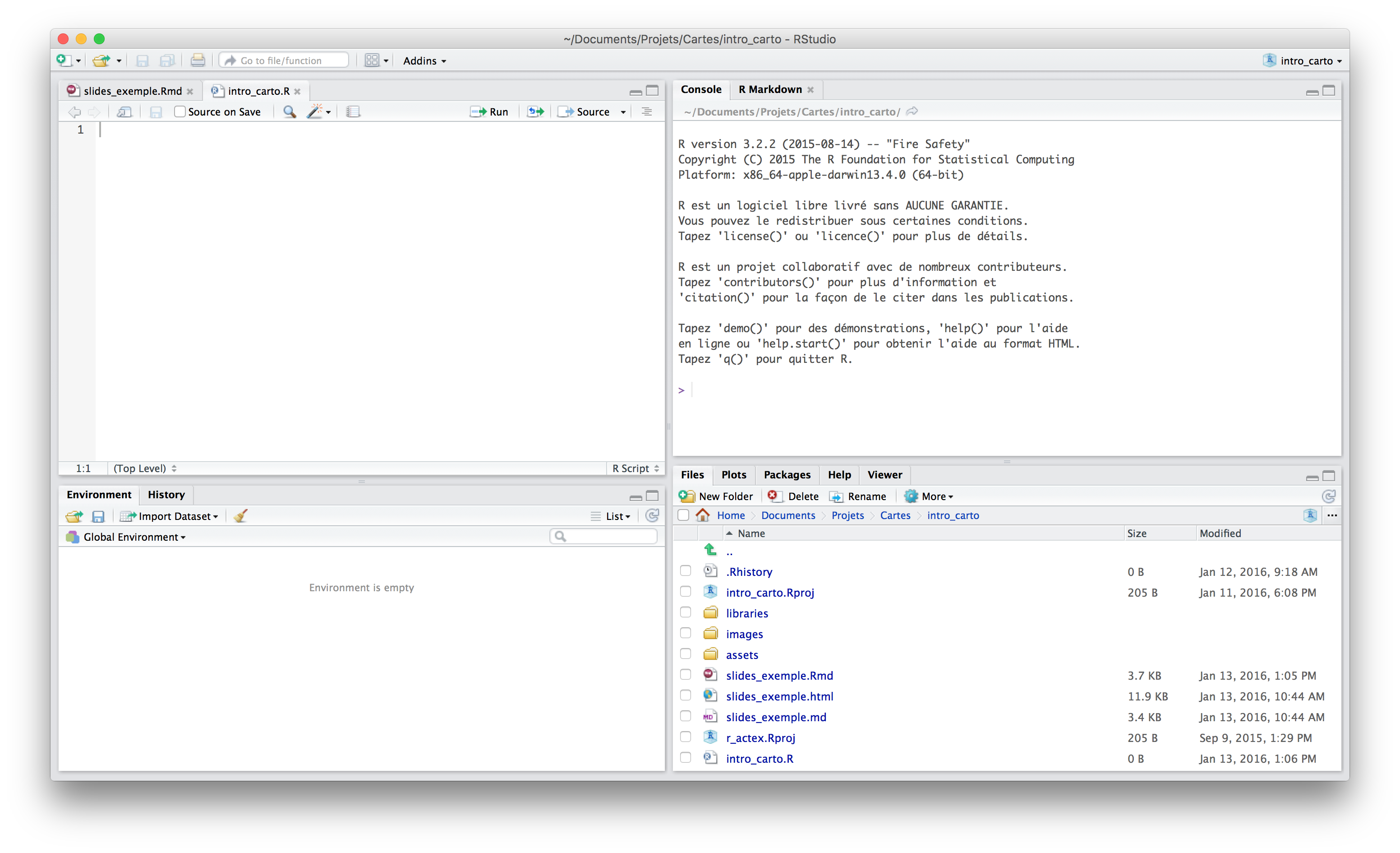
The Console
The console acts like a calculator: one submits a code, it is evaluated and R an answer is returned
2+1
## [1] 3
- If this code is written in the console, just hit "Enter" to evaluate the expression
- If it is written in a script, hit
CTRL + r,CTRL + ENTERorCMD ENTER
Assign a Value to a Name
- To save the result from the evaluation of an expression, R offers two ways:
- an arrow:
<-or->(the latter is not often used) - the equal sign:
=(not my favourite practice)
- an arrow:
- The syntax is the following:
variable_name <- value
a <- 2+1
# Or : a = 2+1 (note that the # sign enables to comment the rest of the line)
Assign a Value to a Name
- To access the value stored in the object, just name it:
a
## [1] 3
a+1
## [1] 4
Changing the value of an object
- The arrow is also used to change the value of an object:
(a <- 2^2)
## [1] 4
- Modifications made to a copy have no impact on the original object:
b <- a ; b <- 20
a ; b
## [1] 4
## [1] 20
Removing an Object
The rm() function removes an object from a specific environment:
a
## [1] 4
rm(a)
a
## Error in eval(expr, envir, enclos): object 'a' not found
Packages
- R packages contain:
- functions
- help files
- possibly data
- The package
basecontains elementary functions (e.g.sum(),mean(),c(), etc.)
Packages
- Some packages are loaded by default
- Others must be installed once and then loaded at each new session
- To install a package, the syntax is:
install.packages("package_name")
- To load a package, the syntax is:
library(package_name)
- RStudio offers a way to easily update packages, in the "Packages" tab
Getting Help
- Widely used packages offer details help files
- Using the function
help("function_name")redirects to the help page offunction_name:
help("log")
?log
- To look some documentation up by a key word, R offers the
help.search()function:
help.search("logarithm")
??logarithm
- The list of keywords is available here: https://svn.r-project.org/R/trunk/doc/KEYWORDS
How to Manipulate Data
Data
- In R, every object has four characteristics:
- a name
- a mode
- a length
- a content
- There are three main modes:
numeric,character,logical
Data type: numeric
- There are two types of
numeric:integersdoubleorreal
a <- 2.0
typeof(a)
## [1] "double"
is.integer(a)
## [1] FALSE
b <- 2
Data type: numeric
typeof(b)
## [1] "double"
c <- as.integer(b)
typeof(c)
## [1] "integer"
is.numeric(c)
## [1] TRUE
Data type: character
- Character objects are defined using simple or double quotes:
a <- "Hello world!"
a
## [1] "Hello world!"
typeof(a)
## [1] "character"
Data type: logical
- If R needs to convert logical to numeric,
TRUEequals1ansFALSEequals0
TRUE + TRUE + FALSE + TRUE*TRUE
## [1] 3
Data length
- The
length()function returns the number of elements contained in an object
a <- 1
length(a)
## [1] 1
- In the example above,
ais a vector that contains a single element - Hence the presence of
[1]in the output
Missing Data
- In R, missing data are represented by the
NAvalue (Not Available) NAs arelogical
x <- NA
typeof(x)
## [1] "logical"
is.na(x)
## [1] TRUE
NULL Object
- The NULL object in R is called
NULL - Its mode is
NULL - Its length is
0
x <- NULL
length(x)
## [1] 0
is.null(x)
## [1] TRUE
Structures
- R offers different structures to organise data
- The main strucures are:
- vector
- factor
- matrix
- list
- data.frame
- We will focus on vectors, factors and data.frame in this document
Structures: Vectors
- Vectors are the main objects in R
- Each element contained in a vector must have the same type
- The
c()function can be used to create a vector:
c(1,2,3)
## [1] 1 2 3
- A name can be assigned to the elements of a vector, a priori or a posteriori
Structures: Vectors
a <- c(last_name = "Piketty", first_name = "Thomas", birth = "1971")
a
##  last_name first_name      birth
##  "Piketty"   "Thomas"     "1971"
b <- c("Piketty", "Thomas", "1971")
b
## [1] "Piketty" "Thomas" "1971"
names(b) <- c("last_name", "first_name", "birth")
b
##  last_name first_name      birth
##  "Piketty"   "Thomas"     "1971"
Structures: Vectors
- In case of different types, R tries to convert the items in the most general type:
c("two", 1, TRUE)
## [1] "two" "1" "TRUE"
Structures: Factors
- Factors are useful for qualitative data
- To create factors, R provides the function
factor():
countries <- factor(c("France", "France", "China", "Spain", "China"))
countries
## [1] France France China  Spain  China
## Levels: China France Spain
class(countries)
## [1] "factor"
Structures: Factors
- To access the levels attributes of a variable:
levels():
levels(countries)
## [1] "China" "France" "Spain"
- The
relevel()function enables to change the reference:
countries <- relevel(countries, ref = "Spain")
countries
## [1] France France China  Spain  China
## Levels: Spain China France
Structures: Ordered Factors
- To order the levels:
ordered():
income <- ordered(c("<1500", ">2000", ">2000", "1500-2000",
                     ">2000", "<1500"),
                   levels = c("<1500", "1500-2000", ">2000"))
income
## [1] <1500     >2000     >2000     1500-2000 >2000     <1500
## Levels: <1500 < 1500-2000 < >2000
Structures: Data Frames
- In Economics, this might be the most frequent structure we use
data.frameobjects are lists of vectors- Each column is a vector: the mode inside each column needs to be the same of all observation
- The
data.frame()function is used to create adata.frame
women <- data.frame(height = c(58, 59, 60, 61, 62, 63, 64, 65,
                                66, 67, 68, 69, 70, 71, 72),
                     weight = c(115, 117, 120, 123, 126, 129, 132,
                                135, 139, 142, 146, 150, 154, 159, 164))
Structures: Data Frames
head(women)
##   height weight
## 1     58    115
## 2     59    117
## 3     60    120
## 4     61    123
## 5     62    126
## 6     63    129
class(women)
## [1] "data.frame"
Structures: Data Frames
dim(women)
## [1] 15 2
nrow(women)
## [1] 15
ncol(women)
## [1] 2
Import Data
- Whatever the type of data, there is probably a function to import it in the R session
- With ASCII files, the two main functions are
read.table()ansscan() - We will not present the
scan()function here - With other type of files, one needs to load a specific library
Import Data: read.table()
- The
read.table()function is designed for data already organized as a table - The output is a
data.frame - Here are the main parameters I use:
| Argument | Description |
|---|---|
file |
File name, or complete path to file (can be an URL) |
header |
Whether the file contains the names of the variables at its first line ? (FALSE by default) |
sep |
Field separator character (white character by default) |
dec |
Character used for decimal points ("." by default) |
na.strings |
Character vector of strungs to be interpreded as NA (NA by default) |
Import Data from Excel Files
- I mainly use two functions:
read.xls()from thegdatapackageread_excel()from thereadxlpackage
- For convenience, we will use the
iris.xlsfile contained in the folder of thegdatapackage
library(gdata)
xlsfile <- file.path(path.package("gdata"), "xls", "iris.xls")
iris <- read.xls(xlsfile) # Creates a temporary csv file
- By default, the first sheet is imported. The
sheetargument enables to import another sheet, either by giving the number or the name of the sheet - The
read_excel()function is faster, has almost the same names for the arguments, but is not as robust at the moment as theread.xls()function. In addition, it returns atbl_dfobject, not adata.frame
Export Data from R
- The function
write.table()can be used to export adata.frameobject (or a matrix) to an ASCII file:
write.table(my_data_frame, file = "file_name.txt", sep = ";")
- To save one or more objects as is:
save(); to import the object(s) back:load():
save(obj_1, obj_2, file = "my_file.rda")
load("my_file.rda")
- To save the entire session:
save.image(); to load the session:load()
save.image("my_session.rda")
load("my_session.rda")
Access elements of a vector
- Elements of a vector can be accessed by their numerical index or by their name (if they are provided with one)
- This can be done by the
"["()function - The arguments of this function are the vector one wants to extract data from and a numerical vector which contains the positions of the elements one wants to extract (or not), or a logical vector (mask)
- As it might be painful to write this function, R provides a shortcut to use the
"["()function:
x <- c(4, 7, 3, 5, 0)
"["(x, 2)
## [1] 7
Access elements of a vector
x[2] # The second element of x
## [1] 7
x[-2] # All the elements of x minus the second one
## [1] 4 3 5 0
x[3:5] # Elements of x from 3rd to 5th position
## [1] 3 5 0
Access elements of a vector
i <- 3:5 ; x[i] # Elements of x from 3rd to 5th position
## [1] 3 5 0
x[c(F, T, F, F, F)] # Second element from x
## [1] 7
x[x<1] # Elements of x that are lower than 1
## [1] 0
x<1 # Returns a logical vector
## [1] FALSE FALSE FALSE FALSE TRUE
Access elements of a vector
- To extract the positions of
TRUEvalues from a logical vector:which() - To extract the positions of the first minimum (maximum) of a logical or numerical vector:
which.min()(which.max())
x <- c(2, 4, 5, 1, 7, 6)
which(x < 7 & x > 2)
## [1] 2 3 6
which.min(x)
## [1] 4
Access elements of a vector
which.max(x)
## [1] 5
x[which.max(x)]
## [1] 7
Modify elements of a vector
- Simply use the
<-symbol
x <- seq_len(5)
x[2] <- 3
x
## [1] 1 3 3 4 5
- Multiple elements can be modified using one instruction
x[2] <- x[3] <- 0
x
## [1] 1 0 0 4 5
Access elements of a matrix or data.frame
- The same function
"["()works - One just needs to indicate the rows (
i) and columns (j) indices:x[i,j]
(x <- matrix(1:9, ncol = 3, nrow = 3))
##      [,1] [,2] [,3]
## [1,]    1    4    7
## [2,]    2    5    8
## [3,]    3    6    9
x[1, 2]
## [1] 4
Access elements of a matrix or data.frame
iandjcan be vectors of length greater than one:
i <- c(1,3) ; j <- 3
x[i,j]  # Elements of first and third row for the third column
## [1] 7 9
- Not providing
ireturns all lines for thejcolumns - Not providing
jreturns all columns for theirows
x[, 2] # Elements of the second column
## [1] 4 5 6
Access elements of a matrix or data.frame
- As for vectors, negative values indicate positions one does not want:
x[, -c(1,3)] # x without first and third columns
## [1] 4 5 6
Access elements of a matrix or data.frame
- In the case of a
data.frame, columns are named and can thus be accessed using these names
women <-data.frame(height =c(58, 59, 60, 61, 62, 63, 64,
                              65, 66, 67, 68,69, 70, 71, 72),
                    weight =c(115, 117, 120, 123, 126, 129, 132, 135,
                              139,142, 146, 150, 154, 159, 164))
colnames(women) # Names of the columns
## [1] "height" "weight"
rownames(women) # Names of the rows
##  [1] "1"  "2"  "3"  "4"  "5"  "6"  "7"  "8"  "9"  "10" "11" "12" "13" "14"
## [15] "15"
Access elements of a matrix or data.frame
dimnames(women) # Names of both rows and columns
## [[1]]
##  [1] "1"  "2"  "3"  "4"  "5"  "6"  "7"  "8"  "9"  "10" "11" "12" "13" "14"
## [15] "15"
##
## [[2]]
## [1] "height" "weight"
Access elements of a matrix or data.frame
- To access a specific column:
$:
women$height
## [1] 58 59 60 61 62 63 64 65 66 67 68 69 70 71 72
Data manipulation with dplyr
- The packeg
dplyroffers many functions that are really easy to use to manipulate data - We will also use the pipe (
%>%) operator (from the packagemagrittr), which transmits a value as the first argument of the following function - For instance :
library(magrittr)
mean(x) %>% log()
- Computes the mean of the object
xand the apply the logarithm function to the result ofmean(x). It can also be written in the following (but harder to read) way:
log(mean(x))
## [1] 1.609438
Data manipulation with dplyr: selection
- To select columns from a
data.frame:select()
library(dplyr)
women %>%
  select(height)
##    height
## 1      58
## 2      59
## 3      60
## 4      61
## 5      62
## 6      63
## 7      64
## 8      65
## 9      66
## 10     67
## 11     68
## 12     69
## 13     70
## 14     71
## 15     72
Data manipulation with dplyr: selection
- To remove a columns from a
data.frame:select()and a negative sign
library(dplyr)
women %>%
  select(-height) %>%
  head()
##   weight
## 1    115
## 2    117
## 3    120
## 4    123
## 5    126
## 6    129
Data manipulation with dplyr: selection
- To select rows according to their position:
slice()
women %>% slice(4:5)
##   height weight
## 1     61    123
## 2     62    126
Data manipulation with dplyr: filtering
- To return rows with matchin conditions:
filter()
women %>%
  filter(height == 60)
##   height weight
## 1     60    120
women %>%
  filter(weight > 120, height <= 62)
##   height weight
## 1     61    123
## 2     62    126
Data manipulation with dplyr: column modifications
- To rename a column:
rename(data, new_name_1 = old_name_1, new_name_2 = old_name_2)
women <-
  women %>%
  rename(masse = weight)
head(women)
##   height masse
## 1     58   115
## 2     59   117
## 3     60   120
## 4     61   123
## 5     62   126
## 6     63   129
Data manipulation with dplyr: column modifications
- Let us create another
data.frame:
unemp <- data.frame(year = 2012:2008,
                    unemployed = c(2.811, 2.604, 2.635, 2.573, 2.064),
                    active_pop = c(28.328, 28.147, 28.157, 28.074, 27.813))
Data manipulation with dplyr: column modifications
- To modify (or create) columns:
mutate()
unemp <-
  unemp %>%
  mutate(unemp_rate = unemployed/active_pop*100,
         log_unemployed = log(unemployed),
         year = year / 1000)
head(unemp)
##    year unemployed active_pop unemp_rate log_unemployed
## 1 2.012      2.811     28.328   9.923044      1.0335403
## 2 2.011      2.604     28.147   9.251430      0.9570487
## 3 2.010      2.635     28.157   9.358241      0.9688832
## 4 2.009      2.573     28.074   9.165064      0.9450725
## 5 2.008      2.064     27.813   7.420990      0.7246458
Data manipulation with dplyr: ordering
- Let us create another
data.frame:
df <- data.frame(last_name = c("Durand", "Martin",
                               "Martin", "Martin", "Durand"),
                 first_name = c("Sonia", "Serge", "Julien-Yacine",
                                "Victor", "Emma"),
                 grade = c(23, 18, 17, 17, 19))
Data manipulation with dplyr: ordering
- To order observations according to one or multiple values:
order():
df %>% arrange(first_name, last_name)
##   last_name    first_name grade
## 1    Durand          Emma    19
## 2    Martin Julien-Yacine    17
## 3    Martin         Serge    18
## 4    Durand         Sonia    23
## 5    Martin        Victor    17
- To order by decreasing values:
desc()(negative sign can be used for numeric columns)
df %>% arrange(first_name, desc(last_name))
##   last_name    first_name grade
## 1    Durand          Emma    19
## 2    Martin Julien-Yacine    17
## 3    Martin         Serge    18
## 4    Durand         Sonia    23
## 5    Martin        Victor    17
Data manipulation with dplyr: joining two data.frame
- Functions to join
data.framesfromdplyrhave an easy syntax:
xxx_join(x, y, by = NULL, copy = FALSE, ...)
xandyare the two tables to joinbyis a character vector containing variables used to join the tables (if ommited, a natural join using all variables with common names accross the two tables will be done)
Data manipulation with dplyr: joining two data.frame
- Let us create two
data.frameto illustrate the different join functions:
exportations <- data.frame(year = 2011:2013,
                           exportations = c(572.6, 587.3, 597.8))
importations <- data.frame(annee = 2010:2012,
                           importations = c(558.1, 625.3,628.5))
Data manipulation with dplyr: joining two data.frame
inner_join(): return all rows fromxwhere there are matching values inx, and all columns fromxandy. If there are multiple matches betweenxandy, all combination of the matches are returned
exportations %>%
  inner_join(importations, by = c(year = "annee"))
##   year exportations importations
## 1 2011        572.6        625.3
## 2 2012        587.3        628.5
Data manipulation with dplyr: joining two data.frame
left_join(): return all rows fromx, and all columns fromxandy. Rows inxwith no match inywill haveNAvalues in the new columns. If there are multiple matches betweenxandy, all combinations of the matches are returned
exportations %>%
  left_join(importations, by = c(year = "annee"))
##   year exportations importations
## 1 2011        572.6        625.3
## 2 2012        587.3        628.5
## 3 2013        597.8           NA
Data manipulation with dplyr: joining two data.frame
right_join(): return all rows fromy, and all columns fromxandy. Rows inywith no match inxwill haveNAvalues in the new columns. If there are multiple matches betweenxandy, all combinations of the matches are returned
exportations %>%
  right_join(importations, by = c(year = "annee"))
##   year exportations importations
## 1 2010           NA        558.1
## 2 2011        572.6        625.3
## 3 2012        587.3        628.5
Data manipulation with dplyr: joining two data.frame
semi_join(): return all rows fromxwhere there are matching values iny, keeping just columns fromx
exportations %>%
  semi_join(importations, by = c(year = "annee"))
##   year exportations
## 1 2011        572.6
## 2 2012        587.3
Data manipulation with dplyr: joining two data.frame
anti_join(): return all rows fromxwhere there are not matching values iny, keeping just columns fromx.
exportations %>%
  anti_join(importations, by = c(year = "annee"))
##   year exportations
## 1 2013        597.8
Data manipulation with dplyr: joining two data.frame
full_join(): return all rows and all columns from bothxandy. Where there are not matching values, returnsNAfor the one missing
exportations %>%
  full_join(importations, by = c(year = "annee"))
##   year exportations importations
## 1 2011        572.6        625.3
## 2 2012        587.3        628.5
## 3 2013        597.8           NA
## 4 2010           NA        558.1
Data manipulation with dplyr: aggregation
- To aggregate data,
dplyroffers an easy way:summarise() - The arguments are a
data.frameand one or multiple operations to do on thedata.frame - Let us create some dummy observations:
# Nombre d'ingenieurs et cadres au chômage
chomage <- data.frame(region = rep(c(rep("Bretagne", 4),
                                     rep("Corse", 2)), 2),
                      departement = rep(c("Cotes-d'Armor", "Finistere",
                                          "Ille-et-Vilaine", "Morbihan",
                                          "Corse-du-Sud", "Haute-Corse"), 2),
                      annee = rep(c(2011, 2010), each = 6),
                      ouvriers = c(8738, 12701, 11390, 10228, 975, 1297,
                                   8113, 12258, 10897, 9617, 936, 1220),
                      ingenieurs = c(1420, 2530, 3986, 2025, 259, 254,
                                     1334, 2401, 3776, 1979, 253, 241))
Data manipulation with dplyr: aggregation
- If we want to compute the mean and standard deviation for the colums
ouvriersandingenieurs:
chomage %>%
  summarise(moy_ouvriers = mean(ouvriers),
            sd_ouvriers = sd(ouvriers),
            moy_ingenieurs = mean(ingenieurs),
            sd_ingenieurs = sd(ingenieurs))
##   moy_ouvriers sd_ouvriers moy_ingenieurs sd_ingenieurs
## 1     7364.167    4801.029       1704.833      1331.482
Data manipulation with dplyr: aggregation
- It is really simple to aggregate data on groups of observations, thanks to the
group_by()function - We just need to first group the data according to some values taken by one or multiple variables, and then apply the aggregation to the result:
chomage %>%
  group_by(annee) %>%
  summarise(ouvriers = sum(ouvriers),
            ingenieurs = sum(ingenieurs))
## Source: local data frame [2 x 3]
##
##   annee ouvriers ingenieurs
##   (dbl)    (dbl)      (dbl)
## 1  2010    43041       9984
## 2  2011    45329      10474
Data manipulation with dplyr: aggregation
- With groups depending on combination of variables:
chomage %>%
  group_by(annee, region) %>%
  summarise(ouvriers = sum(ouvriers),
            ingenieurs = sum(ingenieurs))
## Source: local data frame [4 x 4]
## Groups: annee [?]
##
##   annee   region ouvriers ingenieurs
##   (dbl)   (fctr)    (dbl)      (dbl)
## 1  2010 Bretagne    40885       9490
## 2  2010    Corse     2156        494
## 3  2011 Bretagne    43057       9961
## 4  2011    Corse     2272        513
Data manipulation: tidyr
- The package
tidyrcontains interesting functions to manipulate data - These functions are really important when one realise graphs with ggplot2
- Unfortunately, their use is not as straightforward as the functions from the
dplyrpackage - We will only focus on two functions here:
gather()andspread() - These functions are useful to turn a large table to a long one, and reciprocally
Data manipulation: from a large table to a long one
- First, let us create some dummy data:
pop <- data.frame(city = c("Paris", "Paris", "Lyon", "Lyon"),
                  arrondissement = c(1, 2, 1, 2),
                  pop_municipale = c(17443, 22927, 28932, 30575),
                  pop_all = c(17620, 23102, 29874, 31131))
Data manipulation: from a large table to a long one
- The
gather()function takes adata.frameas its first argument - The second argument (
key) is the name we want to give to the column that will contain the the names of the columns we want to gather, as a factor - The third argument (
value) is the name we want to give to the column that will contain the corresponding values - Then, we need to specify which colums to gather (either by giving or excluding variable names, as in the
select()function)
Data manipulation: from a large table to a long one
library(tidyr)
pop_long <-
  pop %>%
  gather(key = type_pop,
         value = population,
         pop_municipale,pop_all)
pop_long
##    city arrondissement       type_pop population
## 1 Paris              1 pop_municipale      17443
## 2 Paris              2 pop_municipale      22927
## 3  Lyon              1 pop_municipale      28932
## 4  Lyon              2 pop_municipale      30575
## 5 Paris              1        pop_all      17620
## 6 Paris              2        pop_all      23102
## 7  Lyon              1        pop_all      29874
## 8  Lyon              2        pop_all      31131
Data manipulation: from a long table to large one
- Now to go from a long table to a large one:
spread() - The first argument is the
data.frame - The second argument is the name of the colum that contains values that can be converted to a factor. Each level of the factor will end up as a column name
- The third argument is the name of the column that contains the values
Data manipulation: from a long table to large one
pop_long %>%
  spread(type_pop, population)
##    city arrondissement pop_municipale pop_all
## 1  Lyon              1          28932   29874
## 2  Lyon              2          30575   31131
## 3 Paris              1          17443   17620
## 4 Paris              2          22927   23102
The Basics of Graphics with ggplot2
Graphing with ggplot2
- There are several ways to do graphics in R
- We will only focus on ggplot2 here
- And only on the very basic stuff
Graphing with ggplot2
ggplot2 is a plotting system for R, based on the grammar of graphics, which tries to take the good parts of base and lattice graphics and none of the bad parts. It takes care of many of the fiddly details that make plotting a hassle (like drawing legends) as well as providing a powerful model of graphics that makes it easy to produce complex multi-layered graphics. (http://ggplot2.org/)
- Graphics with
ggplot2are layered based - The first layer contains the data
- The other layers contain information to format and plot them
Graphing with ggplot2
- The grammar creates a map that enables to go from data to aesthetics (colour, shape, size, etc.) of geometry (points, lines, polygons, etc.)
- It also enables to transform data
- Or also to do faceting
- Your best friend when using ggplot2 is the online help: http://docs.ggplot2.org/current/
Graphing with ggplot2: structure
- The elements of ggplot2 grammar are:
- raw data (
data) - a graphical projection (
mapping) - some geometries (
geom) - some statistical operations (
stat) - some scales (
scale) - a coordinate system (
coord) - a faceting (
facet)
- raw data (
Graphing with ggplot2: syntax
- The syntax begins with a call to the
ggplot()function - Layers are added thanks to the
+symbol
ggplot(data, aes(x, y, ...)) + layers
- data must be given as a
data.frame
Graphing with ggplot2: an example
- Let us get some data about 135 movies (source: freebase)
load(url("http://egallic.fr/R/films.rda"))
name: name of the filminitial_release_date: release dateruntime: runtimeyear: year of filmingestimated_budget: estimated budgetgross_revenue: gross revenuecountry: first country given in the list of locationscountry_abr: country code
Graphing with ggplot2: an example
- Let us create a narrower
data.framethat focuses only on some countries:
country_list <- c("United States of America", "New Zealand",
                  "United Kingdom", "Spain")
films_s <- films %>%
  filter(country %in% country_list)
Graphing with ggplot2: an example
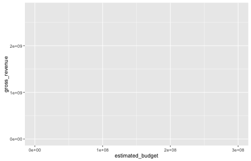
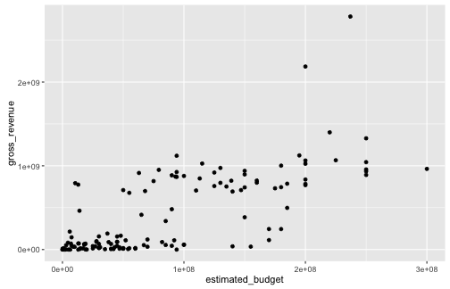
- Let us create a scatterplot representing gross revenue as a function of estimated budget
library(ggplot2)
ggplot(data = films, aes(x = estimated_budget, y = gross_revenue))
Graphing with ggplot2: an example
- Since we gave no information about the geometry, none is visible
library(ggplot2)
ggplot(data = films, aes(x = estimated_budget, y = gross_revenue)) +
  geom_point()
Graphing with ggplot2: aesthetics
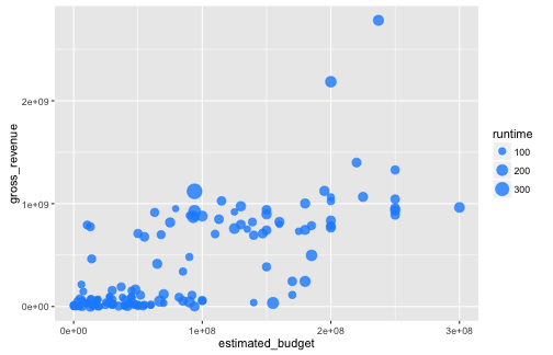
- Now let us play with the aesthetics:
colourshapesizealphafill
- The value of each of the above argument can either:
- be identical to all observations: the argument must be given outside the
aes()function - depend on the value of a variable: the argument must be given inside the
aes()function
- be identical to all observations: the argument must be given outside the
Graphing with ggplot2: aesthetics
ggplot(data = films,
       aes(x = estimated_budget, y = gross_revenue)) +
  geom_point(colour = "dodger blue",
             alpha = .8,
             aes(size = runtime))
Graphing with ggplot2: aesthetics
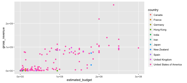
- A scale is associated with each aesthetic
- Whenever it is possible,
ggplot2will merge the scales - For aesthetics depending on the values of a variable, the associated scale will vary according to the type of the variable (
numericalorfactor)
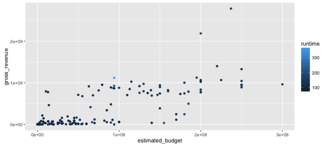
Graphing with ggplot2: aesthetics
ggplot() +
  geom_point(data = films,
             aes(x = estimated_budget,
                 y = gross_revenue, col = runtime))
Graphing with ggplot2: aesthetics
ggplot() +
  geom_point(data = films,
             aes(x = estimated_budget,
                 y = gross_revenue, col = country))

Graphing with ggplot2: aesthetics
ggplot() +
  geom_point(data = films,
             aes(x = estimated_budget,
                 y = gross_revenue, col = country))
Graphing with ggplot2: geometries
- The main geometries are the following:
geom_point()(useful for maps)geom_line()geom_polygon()(useful for maps)geom_path()geom_step()geom_boxplot()geom_jitter()geom_smooth()geom_histogram()geom_bar()geom_density()
Graphing with ggplot2: geometries
geom_*functions have some optionnal parametersdatamappingstatposition
- If these parameters are ommited, they inherit the values from
ggplot()
Graphing with ggplot2: scales
- Let us have a look at the modification of scales
- As we saw, scales are automatically created, but we sometimes need to modify them
- The syntax of scale functions is simple:
- every scale function begins with the prefix
scale_ - It is then followed by the name of the aesthetic (
colour,fill,linetype, ...) - And it ends with the name of the scale (
manual,discrete,gradient, ...)
- every scale function begins with the prefix
Graphing with ggplot2: scales
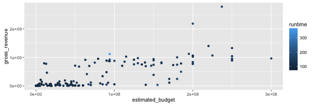
- Let us create a baseline graph:
p <- ggplot(data = films_s,
            aes(x = estimated_budget,
                y = gross_revenue, colour = runtime)) +
  geom_point()
p
Graphing with ggplot2: scales
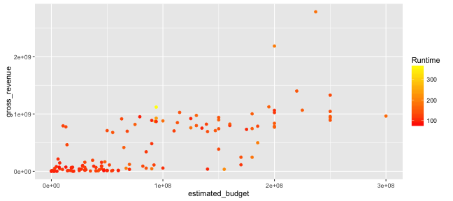
- Let us change the scale so that:
- shorter films are represented in yellow and longer ones in red
- the title of the legend become "Runtime"
p + scale_colour_gradient(name = "Runtime", low = "#FF0000", high ="#FFFF00")
Graphing with ggplot2: scales
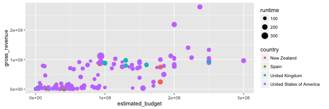
- Now, let the colour of the points vary according to the filming country, and the size of the points vary according to the runtime:
p <- ggplot(data = films_s,
            aes(x = estimated_budget,
                y = gross_revenue,
                colour = country,
                size = runtime)) +
  geom_point()
p
Graphing with ggplot2: scales
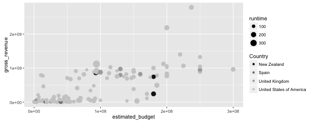
- Let us modify the
colourscale to set it to a grey colour scale:
p + scale_colour_grey(name = "Country",
                      start = .1, end = .8,
                      na.value = "orange")
Graphing with ggplot2: scales
- If we want to define manually the colours associated with the levels of a factor, it is possible
- Note that levels in the legend are arranged in the alphanumerical order: reordering the levels in the
data.framewill change the order in the legend
films_s$country %>% factor() %>% levels()
## [1] "New Zealand"              "Spain"
## [3] "United Kingdom"           "United States of America"
new_order <- c("New Zealand","Spain",
               "United Kingdom",
               "United States of Americz")

films_s <- films_s %>%
  mutate(country = factor(country,
                          levels = new_order))
Graphing with ggplot2: scales
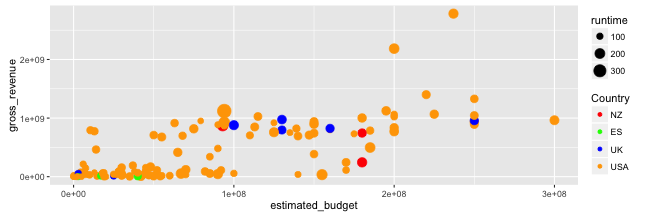
- Now, let us define manually the colours of the points:
(p <- p + scale_colour_manual(name = "Country",
                              values = c("Spain" = "green", "New Zealand" = "red",
                                         "United States of America" = "orange",
                                         "United Kingdom" = "blue"),
                              labels = c("Spain" = "ES", "New Zealand" = "NZ",
                                         "United States of America" = "USA",
                                         "United Kingdom" = "UK")))
Graphing with ggplot2: scales
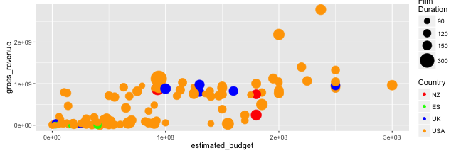
- Let us also change the size of points:
range(films_s$runtime)
## [1] 66 375
p + scale_size_continuous(name = "Film\nDuration",
                          breaks = c(0, 60, 90, 120, 150, 300, Inf),
                          range = c(1,10))
Graphing with ggplot2: groups
ggplot2regroups observation in a bunch of cases- When an aesthetic depends on the values of a variables, it is automatically done
- We can define the groups on our own thanks to the
groupargument in theaes()function
library(reshape2)
df <- data.frame(year = rep(1949:1960, each = 12),
                 month = rep(1:12, 12),
                 passengers = c(AirPassengers))
Graphing with ggplot2: groups
head(df)
##   year month passengers
## 1 1949     1        112
## 2 1949     2        118
## 3 1949     3        132
## 4 1949     4        129
## 5 1949     5        121
## 6 1949     6        135
Graphing with ggplot2: groups
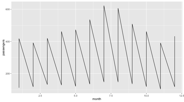
- Without defining groups
ggplot(data = df, aes(x = month, y = passengers)) + geom_line()
Graphing with ggplot2: groups
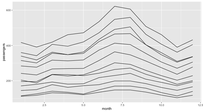
- If we ask to group data according to
year:
ggplot(data = df,
       aes(x = month, y = passengers, group = year)) +
  geom_line()
Graphing with ggplot2: title
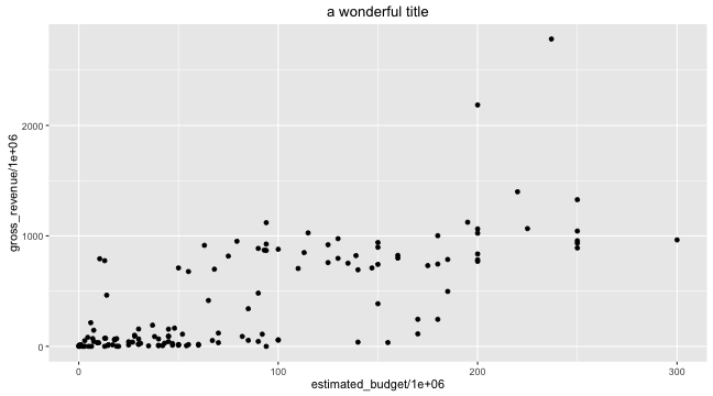
- The title of a graph can be added with the
ggtitle()function, though it might be better practice to leave it blank and leave that to \(\LaTeX\)
ggplot(data = films,
       aes(x = estimated_budget/1e6, y = gross_revenue/1e6)) +
  geom_point() + ggtitle("a wonderful title")
Graphing with ggplot2: axis labels
- The
xlab()andylab()functions enable to modify axis labels
p <- ggplot(data = films,
            aes(x = estimated_budget/1e6, y = gross_revenue/1e6)) +
  geom_point() + ggtitle("Titre") +
  xlab("x axis label") + ylab("y axis label")
Graphing with ggplot2: saving a graph
- To save a graph, just use the
ggsave()function - Precise the name (and path) for the file to create, the plot to save (the plot displayed if the argument is ommited)
- The device to use will be automatically recognized from the file name extension
ggsave(filename = "my_grapg.pdf", plot = p, width = 15, height = 8)
Maps
Print a Map
- We will first create a simple map using data from an R package
- Then we will plot a map from a shapefile
- And then add some external information
rworldmap Package
- A worldmap can be plotted thanks to data contained in the
rworldmappackage - Data are accessed thanks to the
getMap()function - Some data manipulation is necessary to arrange the
data.frameso it can be used byggplot2: we usefortify()to go from aSpatialPolygonsDataFrameto adata.frame
library(ggplot2)
library(rworldmap)
rworldmap Package
worldMap <- getMap()
world_df <- fortify(worldMap)
## Regions defined for each Polygons
head(world_df)
##       long      lat order  hole piece          id         group
## 1 61.21082 35.65007     1 FALSE     1 Afghanistan Afghanistan.1
## 2 62.23065 35.27066     2 FALSE     1 Afghanistan Afghanistan.1
## 3 62.98466 35.40404     3 FALSE     1 Afghanistan Afghanistan.1
## 4 63.19354 35.85717     4 FALSE     1 Afghanistan Afghanistan.1
## 5 63.98290 36.00796     5 FALSE     1 Afghanistan Afghanistan.1
## 6 64.54648 36.31207     6 FALSE     1 Afghanistan Afghanistan.1
rworldmap Package
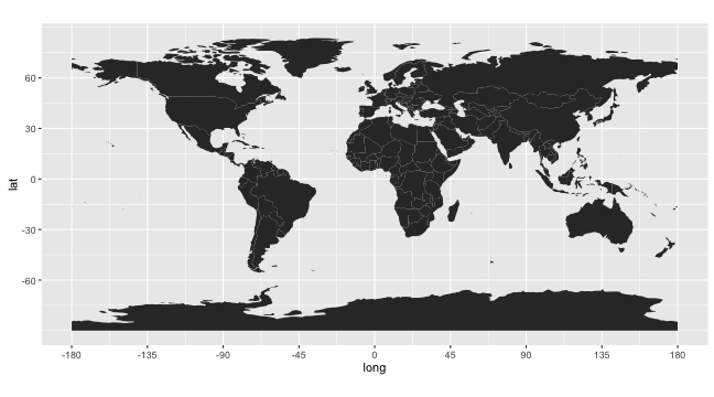
- We just need to precise the mapping, and not to forget the
groupargument to define polygons (otherwise,ggplot2will join all the points together) - We also add a coordinates layer:
coord_quickmap()
worldmap <- ggplot() +
  geom_polygon(data = world_df, aes(x = long, y = lat, group = group)) +
  scale_y_continuous(breaks = (-2:2) * 30) +
  scale_x_continuous(breaks = (-4:4) * 45) +
  coord_equal()
rworldmap Package
worldmap
rworldmap Package
- With the
cord_map()function, we can modify the coordinate system
(worldmap <- ggplot() +
  geom_polygon(data = world_df, aes(x = long, y = lat, group = group)) +
  scale_y_continuous(breaks = (-2:2) * 30) +
  scale_x_continuous(breaks = (-4:4) * 45) +
  coord_map("ortho", orientation=c(61, 90, 0)))

- See examples on Freakonometrics' blog: Moving the North Pole to the Equator
rworldmap Package
rworldmapdata are not very precise. It is useful to do maps at the global scale, but we need to get other data if we want to focus on more specific areas- The
mapspackage contains some other maps with a finer scale - The
map_data()function (fromggplot2) relies on themap()function from the package of the same name - It returns a
data.frame, already arranged to be used byggplot()!
maps Package
- We just need to precise the name of one of the following areas to get the data points:
| Name | Description |
|---|---|
county |
American counties |
france |
France |
italy |
Italy |
nz |
New-Zealand |
state |
United States with all states |
usa |
United States |
world |
World Map |
world2 |
World Map centered on Pacific |
maps Package
- If one wants a specific state for a country, one needs to use the
regionargument
map_fr <- map_data("france")

# Region names
head(unique(map_fr$region))
## [1] "Nord"           "Pas-de-Calais"  "Somme"          "Ardennes"
## [5] "Seine-Maritime" "Aisne"
head(map_fr, 3)
##       long      lat group order region subregion
## 1 2.557093 51.09752     1     1   Nord      <NA>
## 2 2.579995 51.00298     1     2   Nord      <NA>
## 3 2.609101 50.98545     1     3   Nord      <NA>
maps Package
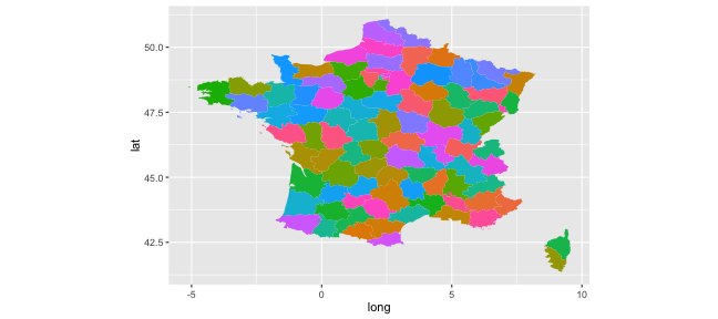
- France map:
(p_map_fr <- ggplot(data = map_fr,
                   aes(x = long, y = lat, group = group, fill = region)) +
  geom_polygon() + coord_equal() + scale_fill_discrete(guide = "none"))
maps Package
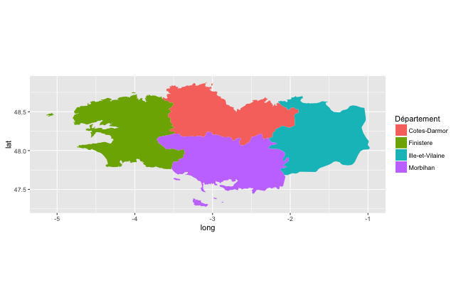
- Brittany map:
library(stringr)
ind_bzh <-
  map_fr$region %>%
  unique() %>%
  str_detect(regex("armor|finis|vilaine|morb",
                   ignore_case = TRUE))

(dep_bzh <- unique(map_fr$region)[ind_bzh])
## [1] "Cotes-Darmor" "Finistere" "Ille-et-Vilaine" "Morbihan"
map_fr_bzh <- map_data("france", region = dep_bzh)
maps Package
(p_map_fr_bzh <-
   ggplot(data = map_fr_bzh,
          aes(x = long, y = lat, group = group, fill = region)) +
  geom_polygon() + coord_equal() + scale_fill_discrete(name = "Département"))
Shapefile
- The
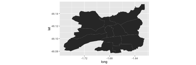
rgdalpackage provides thereadOGR()function that loads data from a shapefile into the R session - For example, let us download Rennes neighbourhoods on data.rennes-metropole.fr
library(rgdal)
library(maptools)
library(ggplot2)
library(dplyr)
Shapefile
# Import shp data
rennes <- readOGR(dsn="./quartiers_shp_lamb93", layer="quartiers")
## OGR data source with driver: ESRI Shapefile
## Source: "./quartiers_shp_lamb93", layer: "quartiers"
## with 12 features
## It has 2 fields
# Change the coordinates
rennes <- spTransform(rennes, CRS("+proj=longlat +ellps=GRS80"))
Shapefile
# Add an ID field
rennes@data$id <- rownames(rennes@data)

# Transform the data so it ends up in a ggplot2-friendly data.frame
rennes_points <- fortify(rennes, region="id")

# To avoid holes
rennes_df <- plyr::join(rennes_points, rennes@data, by="id")
Shapefile
(p_map_rennes <-
   ggplot(data = rennes_df,
          aes(x = long, y = lat, group = group)) +
  geom_polygon() +
  coord_equal())
Choropleth Maps
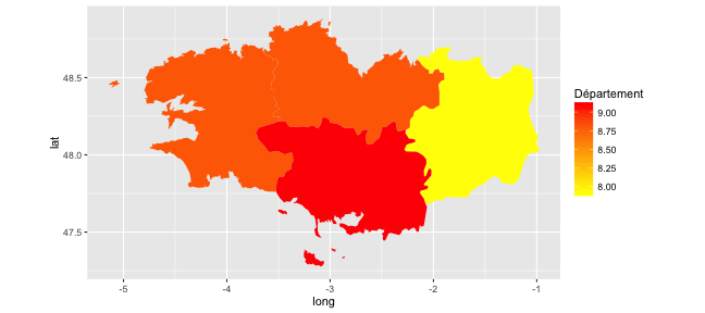
- In choropleth maps, colors of areas correspond to a statistics
- With
ggplot2, it is quite simple: just add a variable to thedata.frame
tx_chomage_2014_T1 <- data.frame(
  region = c("Cotes-Darmor","Finistere",
             "Ille-et-Vilaine", "Morbihan"),
  tx_chomage_2014_T1 = c(8.8, 8.8,7.9, 9.1))

# Add value for tx_chomage_2014_T1 on each line of the data.frame
map_fr_bzh <-
  map_fr_bzh %>%
  left_join(tx_chomage_2014_T1)
Choropleth Maps
- One only needs to precise the
fillaesthetics!
(p_map_fr_bzh <-
   ggplot(data = map_fr_bzh,
          aes(x = long, y = lat, group = group,
              fill = tx_chomage_2014_T1)) +
  geom_polygon() + coord_quickmap() +
  scale_fill_gradient(name = "Département", low ="#FFFF00", high = "#FF0000"))
Choropleth Maps
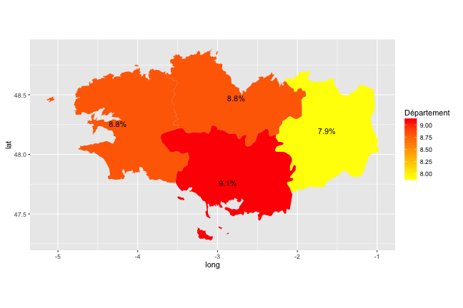
- It is almost straightforward to add annotations:
- First let us find coordinated of median points for each region
# Find the coordinates of the median point
mid_range <- function(x) median(range(x, na.rm = TRUE))

center <-
  map_fr_bzh %>%
  group_by(region) %>%
  dplyr::summarise(long = mid_range(long),
         lat = mid_range(lat))
Choropleth Maps
- Then let us add the unemployment rates:
center <-
  center %>%
  dplyr::left_join(tx_chomage_2014_T1) %>%
  dplyr::mutate(label_unemp = paste0(tx_chomage_2014_T1, "%"))
Choropleth Maps
p_map_fr_bzh + annotate("text", x = center$long,
                        y = center$lat, label = center$label_unemp)
